A coupled level set framework for bladder wall segmentation with application to MR cystography

Abstract

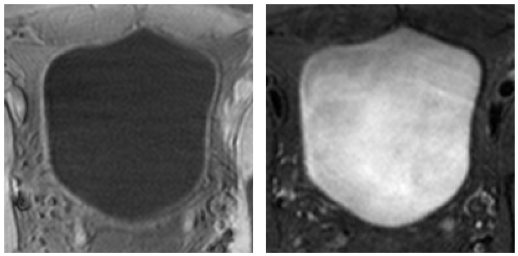
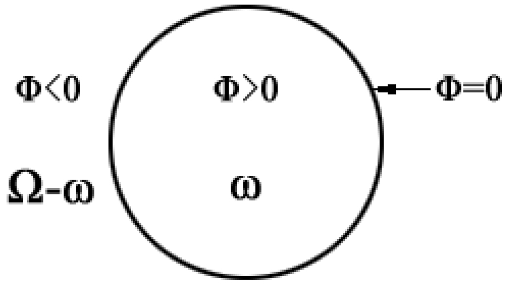
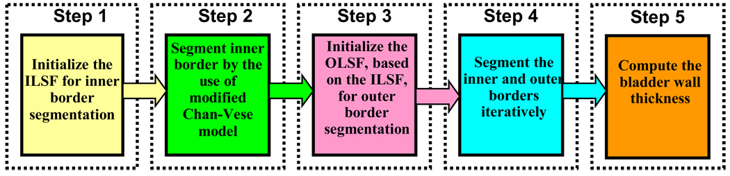
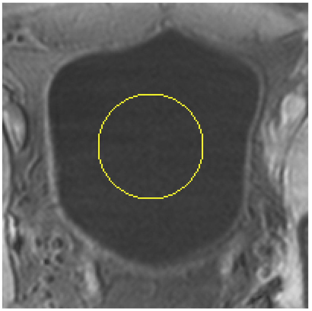
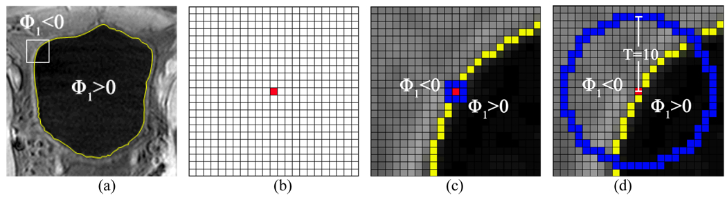
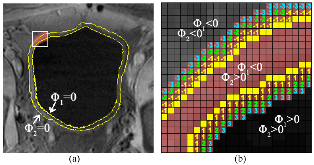
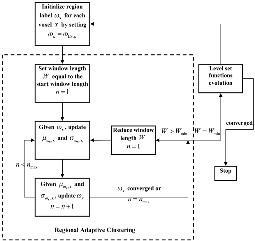
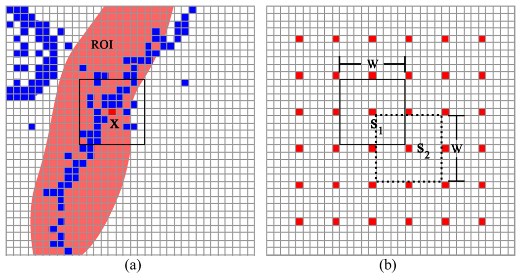
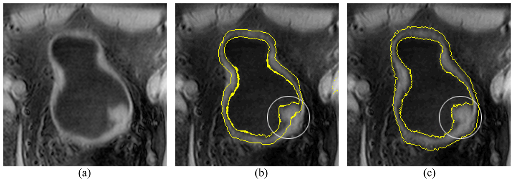
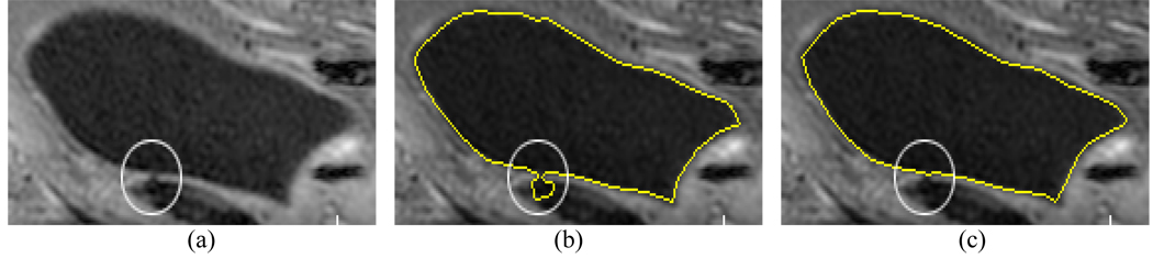
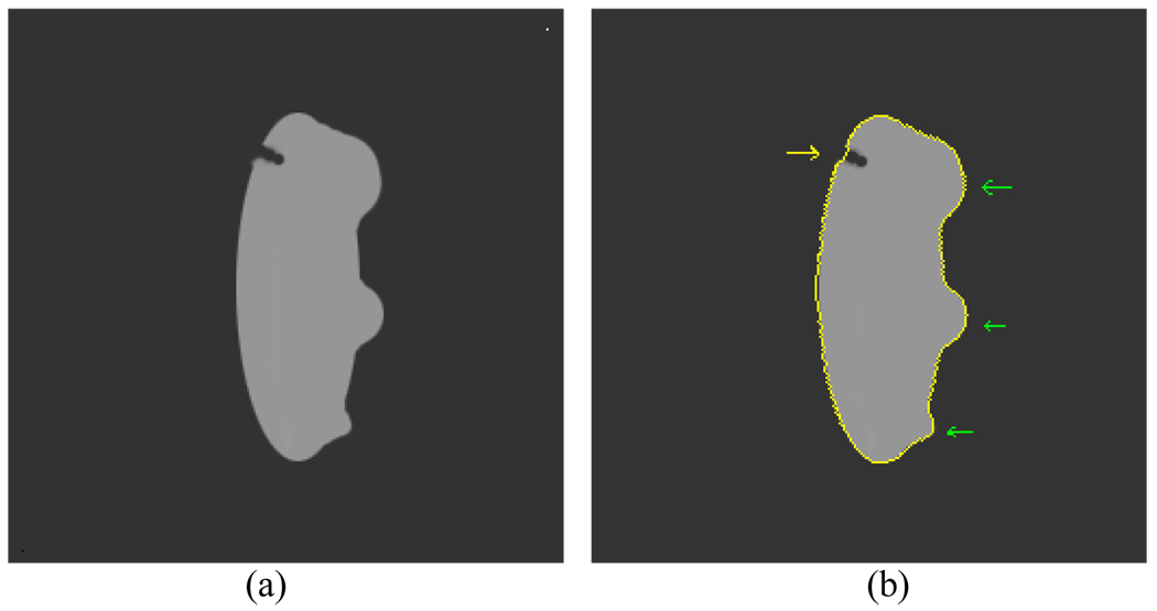
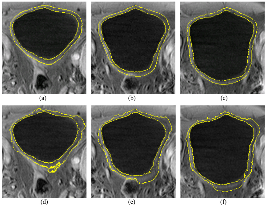
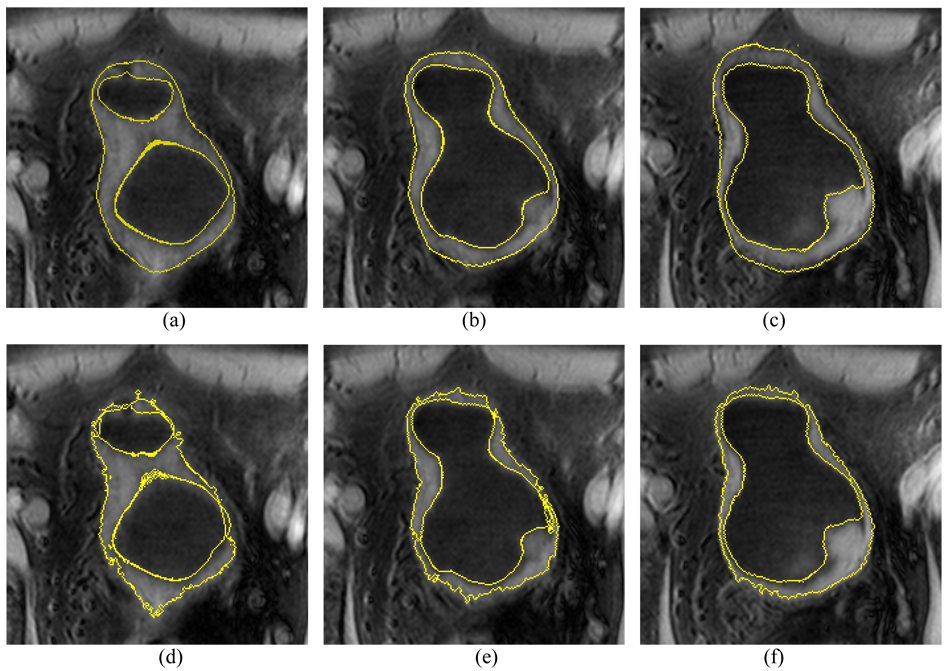
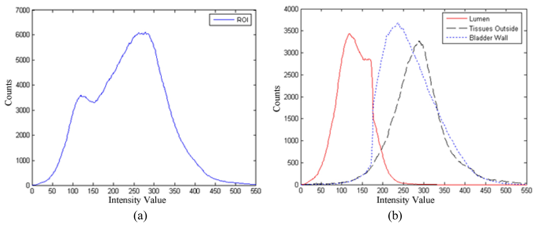
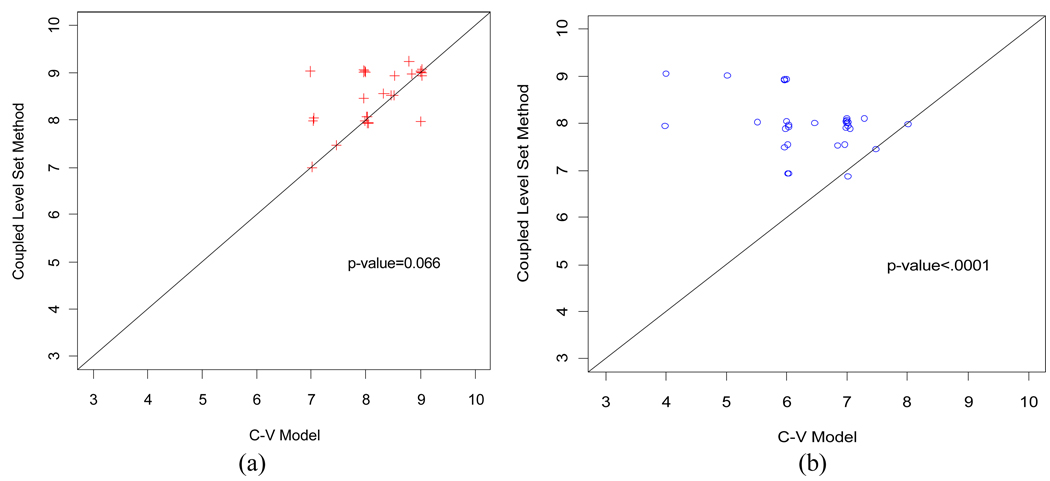
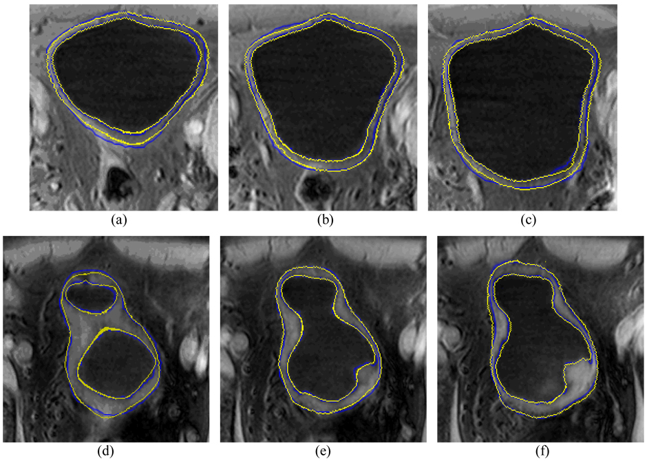
In this paper, we propose a coupled level set (LS) framework for segmentation of bladder wall using T(1)-weighted magnetic resonance (MR) images with clinical applications to virtual cystoscopy (i.e., MR cystography). The framework uses two collaborative LS functions and a regional adaptive clustering algorithm to delineate the bladder wall for the wall thickness measurement on a voxel-by-voxel basis. It is significantly different from most of the pre-existing bladder segmentation work in four aspects. First of all, while most previous work only segments the inner border of the wall or at most manually segments the outer border, our framework extracts both the inner and outer borders automatically except that the initial seed point is given by manual selection. Secondly, it is adaptive to T(1)-weighted images with decreased intensities in urine, as opposed to enhanced intensities in T(2)-weighted scenario and computed tomography. Thirdly, by considering the image global intensity distribution and local intensity contrast, the defined image energy function in the framework is more immune to inhomogeneity effect, motion artifacts and image noise. Finally, the bladder wall thickness is measured by the length of integral path between the two borders which mimic the electric field line between two iso-potential surfaces. The framework was tested on six datasets with comparison to the well-known Chan-Vese (C-V) LS model. Five experts blindly scored the segmented inner and outer borders of the presented framework and the C-V model. The scores demonstrated statistically the improvement in detecting the inner and outer borders.

Fig. 1

Typical examples of T₁-weighted (left) and T₂-weighted (right) MR images of the bladder. The bladder wall is more distinguishable in T₁-weighted image than in T₂-weighted scan.

Fig. 2

An illustration of the level set function and the zero level set surface.

Fig. 3

A flowchart of the coupled level set framework for bladder wall segmentation. It consists of five steps.

Fig. 4

The ZLSS of ILSF is initialized manually inside the bladder lumen as the surface of a small ball. The yellow circle indicates the initialized ZLSS in this slice.

Fig. 5

An example to illustrate the improvement of the bent rate against the curvature term. Picture (a) shows the original T₁-weighted MR bladder image, where yellow curve is the ZLSS of ILSF. The area inside the white square frame contains 23×23 image pixels, which is enlarged in the following illustrations. Picture (b) shows the 23×23 array with the center pixel being marked red. In picture (c), the effective region of curvature is colored blue while the central pixel is colored red. In picture (d) as an example, the effective region of bent rate is a disk-shaped region with radius equal to 10 whose boundary is shown in blue. The red pixel is at the center.

Fig. 6

An illustration of the ROI. Picture (a) shows the original image with ZLSSs in a slice. The yellow curves are the ZLSSs in this slice. Picture (b) is the enlarged region in the white frame in (a). When d = 3 is chosen as an example, the ROI in the white frame includes those voxels which are colored pink, i.e., the ROI includes (1) the space between the yellow lines and (2) the expanded space labeled −3, −2, −1, 1, 2, and 3.

Fig. 7

The flowchart which illustrates the iterative procedure of image energy construction by the use of the RACA and the LS function evolution.

Fig. 8

An illustration of the method for selection of sample voxels and windows to estimate the parameters for each voxel. In picture (a), only the blue voxels in the ROI and the square window are used to estimate the mean and standard deviation for the sampler voxel at location x. Picture (b) shows the discrete sampling and the window alignment.

Fig. 9

An example which shows the influence of the bent rate and the curvature on the initialization of the OLSF. The bent rate is able to effectively flatten the concave surface and gives a better approximation for the outer border than the curvature. Picture (a) is the original image slice. Picture (b) shows the initialization of the OLSF by the use of the curvature. Picture (c) shows the initialization of the OLSF by the use of the bent rate.

Fig. 10

An example which shows the difference of the bent rate and the curvature in preventing ZLSS from leaking out. The bent rate is more controllable and effective than the curvature in preventing leaking. Picture (a) is the original image slice. There is a small gap (due to decreased image intensities) as indicated by the white circle. Picture (b) shows the segmentation result by the use of the curvature. Picture (c) shows the segmentation result by the use of the bent rate.

Fig. 11

An artificial image mimics the bladder wall which shows how the bent rate influences the segmentation result. (a) The original image. (b) The segmentation result. The yellow curve represents the segmentation result. The abnormalities of different sizes on the inner border are pointed by green arrow, while a gap on the outer border is pointed by yellow arrow.

Fig. 12

An example of segmentation results from the volunteer datasets using the presented method and the C-V model. Top row (a)–(c) shows the segmented results of the presented method. Bottom row (d)–(f) shows the segmented results of the C-V model. The intensity distribution is very complex around the outer border of the bladder wall. Since it considers the local contrast and applies prior geometry constraint, the presented method performs much better than the original C-V mode.

Fig. 13

An example of segmentation results from the patient datasets using the presented method and the C-V mode. An abnormal protrusion is included in the slices. Pictures (a)–(c) show the segmented results of the presented method. Picture (d)–(f) show the segmented results of the C-V model. The presented method produces better results than the C-V model.

Fig. 14

Histogram of voxels inside a VOI enclosing the whole bladder of Fig. 12. Picture (a) is the histogram of all voxels inside the VOI. Picture (b) shows the histograms of the segmented voxels inside the VOI as bladder lumen (red), bladder wall (blue), and soft tissues outside the bladder wall (black). The image intensity distributions of the bladder wall and the surrounding soft tissues overlap on a large portion of the histogram.

Fig. 15

Scatter plot of the scores from the coupled-LS method against the C-V model. Picture (a) shows the scatter plot of the scores from the segmented inner border. Picture (b) shows the scatter plot of the scores from the segmented outer border. The coupled-LS method gained significant higher scores than the C-V model, especially for the outer border of the bladder wall.

Fig. 16

Examples of manually-drawn results and computer segmentation results. Top row (a)–(c) shows the results from a volunteer study, where the blue contour represents the manually-drawn result and the yellow contour represents the computer segmentation result of the presented method. The computer segmentations results were also shown in Fig. 12 and Fig. 13. The bottom row (d)–(f) shows the results from a patient study.

Fig. 17

Examples of 3D renderings of a few segmented bladder walls. Picture (a) is an outside view of the segmented outer border of a dataset. Picture (b) is a cut view inside the segmented inner border of the dataset. Picture (c) shows the outside view of the segmented outer border of another dataset. The highlighted yellow patch indicates the area of abnormality. Picture (d) shows the cut view of the segmented inner border of the same dataset with abnormality. The abnormality can be highlighted in the 3D reconstructed bladder because of the thickness variation.

References

-
- Jemal A, Thomas A, Murray T, Thun M. Cancer statistics. A Cancer Journal for Clinicians. 2002;52:23–47. - PubMed
- Shaw ST, Poon SY, Wong ET. Routine urinalysis: is the dipstick enough? The Journal of the American Medical Association. 1985;253:1596–1600. - PubMed
- Lamm DL, Torti FM. Bladder cancer. A Cancer Journal for Clinicians. 1996;46:93–112. - PubMed
- Vining DJ, Zagoria RJ, Liu K, Stelts D. CT cystoscopy: an innovation in bladder imaging. American Journal of Roentgenology. 1996;166:409–410. - PubMed
- Hussain S, Loeffler JA, Babayan RK, Fenlon HM. Thin-section helical computer tomography of the bladder: initial clinical experience with virtual reality imaging. Urology. 1997;50(5):685–689. - PubMed
Publication types
MeSH terms
Substances
Grants and funding
LinkOut - more resources
Full Text Sources
Other Literature Sources