Origin of active states in local neocortical networks during slow sleep oscillation

Abstract

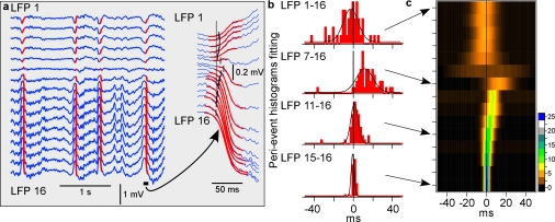
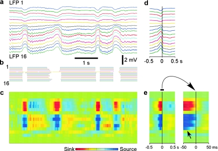
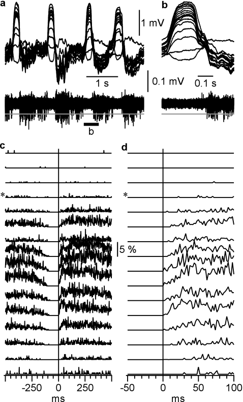
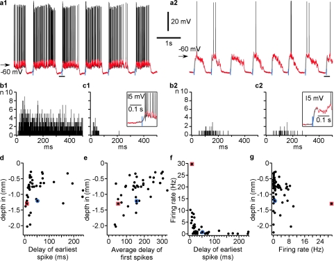
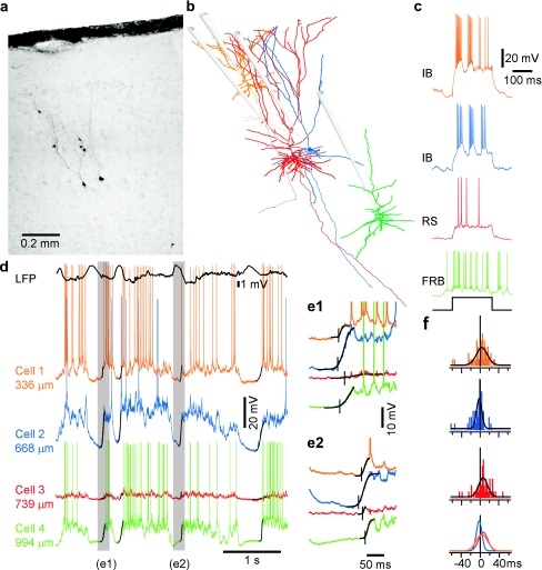
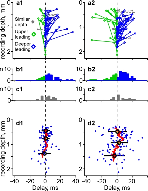
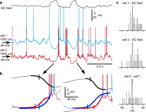
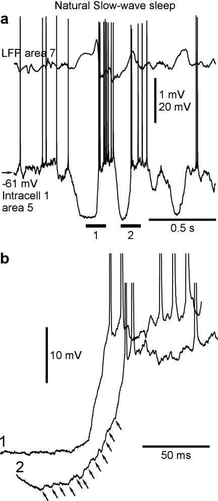
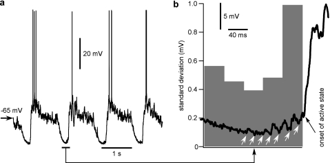
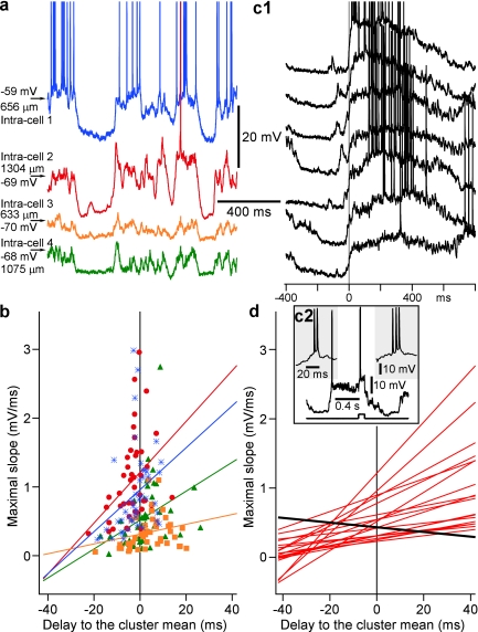
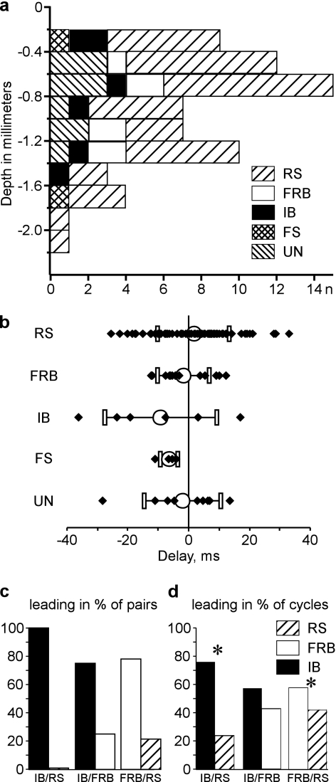
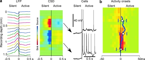
Slow-wave sleep is characterized by spontaneous alternations of activity and silence in corticothalamic networks, but the causes of transition from silence to activity remain unknown. We investigated local mechanisms underlying initiation of activity, using simultaneous multisite field potential, multiunit recordings, and intracellular recordings from 2 to 4 nearby neurons in naturally sleeping or anesthetized cats. We demonstrate that activity may start in any neuron or recording location, with tens of milliseconds delay in other cells and sites. Typically, however, activity originated at deep locations, then involved some superficial cells, but appeared later in the middle of the cortex. Neuronal firing was also found to begin, after the onset of active states, at depths that correspond to cortical layer V. These results support the hypothesis that switch from silence to activity is mediated by spontaneous synaptic events, whereby any neuron may become active first. Due to probabilistic nature of activity onset, the large pyramidal cells from deep cortical layers, which are equipped with the most numerous synaptic inputs and large projection fields, are best suited for switching the whole network into active state.

Figure 1.

Depth profile of the LFP during natural slow-wave sleep. (a) LFPs recorded with a 16-channel Michigan probe, inserted perpendicularly to the cortical surface. Red lines show sigmoidal fits of the transitions from silent state to active states. The point at which a fit reached 10% of its amplitude was taken as the onset time of an active state. One cycle is shown at expanded scale. (b) Histograms of delays of the active state onsets in indicated channels relative to the activity onset in channel 16, taken as the reference. Fifty cycles were used. Black lines show Gaussian fits. (c) Depth profile of active state onsets. For each channel, Gaussian fit of the distribution of activity-onset delays relative to channel 16 is shown, color coded for n cycles as indicated by the scale bar.

Figure 2.

Alternating pattern of current sinks and sources during natural slow-wave sleep revealed with CSD analysis. (a) Depth profile of LFPs recorded with a 16-channel silicon probe inserted perpendicularly to the cortical surface. (b) Active states detected in LFP traces from (a). (c) CSD analysis of the traces from (a). Note alternating pattern of sinks and sources corresponding to the slow waves in the LFP. (d) Depth profile of averaged LFPs during the transition from silent to active states. Mid amplitude in the transition from silent to active states in channel 16 in a 150-s recording segment were taken as reference (zero point in timescale in (d) for calculating averages (n = 101) in all channels. (e) Averaged CSD during the transition from silent to active state, and its central portion at 10-fold higher temporal resolution (right panel). Note that during active states, the flow of current is less pronounced and more variable in terms of spatiotemporal organization of sources and sinks than during silent states.

Figure 3.

Depth distribution of neuronal firing during slow-wave sleep. (a) LFP (top traces) and multiunit activity (bottom trace) recordings at the border of cortical areas 5 and 7 (associative cortex) during short episode of slow-wave sleep. Recordings were performed with a 16-channel silicon probe inserted perpendicularly to the cortical surface. The recording sites were separated by 100 μm, the upper recording site was just below cortical surface. LFP and multiunit activity traces were obtained from the same electrodes, by band-pass filtering 0.1 Hz to 10 kHz and 0.5–10 kHz, respectively. (b) A segment from (a) as indicated by the bar, at higher temporal resolution. (c) Probability distributions of multiunit firing during a cycle of slow oscillation. Pooled data from 290 cycles from 5 different sleep episodes. Spikes were detected as all peaks that exceeded a threshold (gray lines in a and b), set at 5× SD of the noise fluctuations during silent state. * Indicates the electrode at which the polarity of slow waves were reversed. Vertical line shows onset of active state determined in the LFP recorded from the deepest electrode. (d) Zoom in on the silent to active state transition from (c). Note that the first firing occurs in neurons located between 800 and 1200 μm from cortical surface.

Figure 4.

Cells from deep layers fire earlier than other cells at the onset of active state. (a) Intracellular recording from 2 cells in area 7 of cat neocortex, with an exceptionally high firing rate (a1) and low firing rate (a2). Black traces show original recordings, superimposed red traces show the same segment of recordings after removing action potentials. The onset of active states (blue vertical lines) was determined with sigmoid fit (gray line) of the transition from silent to active state, at 10% of the fit amplitude. Insets show enlarged cycles indicated by the horizontal bars in (a). (b) Histograms of all spikes in cells shown in a1 and a2 relative to the active state onset (b1, 49 cycles, b2, 65 cycles). Bin width is 1 ms. (c) Histograms of the first spike delay at onsets of active states. Note that even in the cell with a very high firing rate, the first spike occurred several milliseconds after the onset of cell depolarization. No spikes occurred before the active state (depolarization) started. (d) Cell depth plotted against the delay of the earliest spike from all active states. Note that earliest spike delays in cells located between −1.0 and −1.4 mm were shorter than in other cells. (e) Cell depth plotted against the first spike delay averaged over all active states. Note again that cells from deep layers have a tendency to fire earlier than others. (f) Firing rate of cells plotted against the delay to the earliest spike at the onset of an active state. Note that cells with higher firing rate had shorter earliest spike delays. (g) Cell depth plotted against their firing rate. In (d–g), red square symbols mark data from the cell shown in a1, and blue circle symbols show data from the cell presented in a2.

Figure 5.

Onsets of active states in local neuronal constellations. Data from 4 simultaneously recorded neurons are color coded; each neuron is represented by its own color in b–f. (a) Microphotograph and (b) Neurolucida reconstructions of 4 simultaneously recorded pyramidal cells. The gray neuron was recorded prior to cell-3 (red) with the same electrode. Position of recording electrodes is shown schematically. (c) Responses of the neurons from b to depolarizing current pulses and their electrophysiological identification as IB, RS, and FRB cells. (d) LFP and intracellular activities of 4 simultaneously recorded neurons. Black lines superimposed on membrane potential traces show sigmoid fits of active state onsets. (e) Two periods from d shown at expanded scale. Vertical bars indicate active state onsets. Note the different order of activity onset in neurons in the 2 episodes. (f) Distributions of delays of active state onsets in cells 1–3 relative to the activity onset in cell 4 taken as reference. The lowermost panel shows an overlay of the 3 distributions. Note the negative shift of the cell 2, blue delay distribution, indicating that this IB cell had a tendency to lead in the majority of cycles and the positive shift of histogram for cell 3 (red) indicating that this RS cell was often the last involved in activity.

Figure 6.

Depth profile of activity onset in simultaneously recorded neurons: Population analysis. (a) Dependence of activity onset on the recording depth in cell pairs. Each pair of simultaneously recorded neurons is represented by 2 symbols connected with a line. Y-coordinates show the depth at which the cell was recorded. Delays of activity onsets in the upper cell in a pair were calculated relative to the activity onsets in the deeper cell, taken as reference. Positive delays (blue) indicate pairs with deeper cell leading; negative delays (green) indicate pairs with upper cell leading. Gray indicates recordings with similar depth (vertical difference <100 μm). Left column, analysis of the onsets of active states obtained with the method of sigmoid fits; right column, detection of the beginning of developed active states using the method based on values of membrane potential and its SD. (b,c) Distributions of the delays in cell pairs, color coded as in (a). (d) Dependence of the delay of activity onset in state clusters on recording depth. Each blue diamond symbol represents data for one cell. Running averages (red symbols) were calculated for sets of 17 neurons. For gross averages (cycles, ±SD), cells were segregated in 3 nearly equally populated groups, (d1) above 575 μm (n = 27), between 575 and 1050 μm (n = 27), and deeper than 1050 μm (n = 27). (d2) above 670 μm (n = 36), between 670 and 1100 μm (n = 35), and deeper than 1100 μm (n = 36). Note that, most often, activity started earlier in the deeper neurons.

Figure 7.

The high variability of active state onsets in cells during natural sleep. (a) Simultaneously recorded DC field potential and intracellular activity of 2 closely located (<100 μm in lateral distance) neurons. (b) Two cycles from (a) shown at expanded scale. Action potentials are truncated. The thick line shows sigmoid fits of transitions to active states. Note the opposite order of activity onset in the 2 cells in 2 consecutive cycles. (c) Distributions of the activity-onset delays in the 2 cells relative to the onset of active state in DC field potential and in the simultaneously recorded cell. Note that all distributions cover zero, and thus, in any pair, the opposite orders of activation were encountered, with delays up to 40 ms.

Figure 8.

Progressive buildup versus sharp transitions from silent to active states. (a) Intracellular and LFP recordings during natural slow-wave sleep. (b) Zoom in on active state onsets from 2 consecutive cycles. Note the presence of many individual events (oblique arrows) in the onset with slow development of depolarization (2) and a smooth slope of a rapid transition (1).

Figure 9.

Membrane potential fluctuations increase just before the onset of active state. (a) Intracellular recording in suprasylvian gyrus (area 7) of cat anesthetized with a mixture of ketamine and xylazine. (b) A segment from a is enlarged and superposed on a histogram showing the averaged membrane potential SD (n = 50 cycles, 0 time is active state onset defined with sigmoid fit). Bin width is 40 ms. Note the large increase in the SD of the membrane potential just prior to the active state onset.

Figure 10.

Earlier involvement in activity is associated with slower transitions to active states. (a) A segment of simultaneous quadruple intracellular recording from closely located neurons in area 7, performed under ketamine/xylazine anesthesia. (b) Maximal slope of a transition from silent to active state, estimated from sigmoid fitting, plotted against the delay of the cell relative to the mean onset of activity in the cluster. Each point shows data for one cycle. For each cell, a regression line is shown. Color code corresponds to the 4 cells in (a). Note that in cycles in which activity onset in a cell was earlier than in other cells (negative delays), the slope of transition was smaller, typical for a progressive synaptic buildup. (c1) Examples of transitions from silent to active state in a cell that often showed a strong buildup of depolarization prior to the transition. Zero time is half amplitude of depolarization. The cell was IB, as identified by bursts during both spontaneous activity (left inset in c2) and in responses to depolarizing current pulses (right inset in c2). (d) Relation between maximal slope of transition from silent to active states and the delay of activity onset in the cell relative to the mean onset in the cluster. Regression lines (as in b) for 18 cells. Note that in 17 of 18 neurons, earlier onsets of active state were associated with smaller slopes of transition. The only one cell showing an inverse relation (black line) is illustrated in c.

Figure 11.

IB cells are leading the onset of active states. (a) Depth distribution of different types of neocortical neurons, as indicated by symbols: RS, FRB, IB, and fast spiking (FS). UN—unidentified neurons. Note that neurons of all electrophysiological types were found at any depth. (b) Delay of onsets of clustered active states in cells of different electrophysiological types. (c,d) Activity onset in pairs composed of different cell types. IB cells were leading in all pairs consisting of IB/RS cells (n = 5 pairs), and in 3 of 4 IB/FRB pairs. In these pairs, the IB cells were also leading in most of individual activity cycles (IB/RS: n = 210 cycles; IB/FRB, n = 182 cycles). In FRB/RS pairs, FRB cells were leading in 7 of 9 pairs, and in the majority of cycles (n = 544 cycles). *In (d) indicates significant difference, P < 0.05 to a bilateral binomial test approximated by normal law. For IB/FRB pairs, P = 0.054.

Figure 12.

Comparison of the depth profiles of field potential and intracellular events during slow oscillation. (a) Depth profile of the LFP, CSD, and intracellular activity during transition from silent to active state during natural slow-wave sleep. Arrows show approximate depth of the 2 neurons relative to the CSD profile (LFP and CSD plots are from Fig. 2). (b) Depth profile of the onsets of active states in the LFP (data from Fig. 1) and the running average of active state onsets in intracellularly recorded neurons (data from Fig. 6d2).

References

1. Blake H, Gerard RW. Brain potentials during sleep. Am J Physiol. 1937;119:692–703.
1. Cash SS, Halgren E, Dehghani N, Rossetti AO, Thesen T, Wang C, Devinsky O, Kuzniecky R, Doyle W, Madsen JR, et al. The human K-complex represents an isolated cortical down-state. Science. 2009;324:1084–1087. - PMC - PubMed
1. Chauvette S, Volgushev M, Mukovski M, Timofeev I. Local origin and long-range synchrony of active state in neocortex during slow oscillation. In: Timofeev I, editor. Mechanisms of spontaneous active states in the neocortex. Kerala (India): Research Signpost; 2007. pp. 73–92.
1. Compte A, Sanchez-Vives MV, McCormick DA, Wang X-J. Cellular and network mechanisms of slow oscillatory activity (<1 Hz) and wave propagations in a cortical network model. J Neurophysiol. 2003;89:2707–2725. - PubMed
1. Connors BW, Gutnick MJ. Intrinsic firing patterns of divers neocortical neurons. Trends Neurosci. 1990;13:99–104. - PubMed
Publication types