. 2010 Mar 3;30(9):3531-43.
doi: 10.1523/JNEUROSCI.4911-09.2010.

Predictive coding as a model of response properties in cortical area V1

Affiliations

Predictive coding as a model of response properties in cortical area V1

Michael W Spratling. J Neurosci. .

Abstract

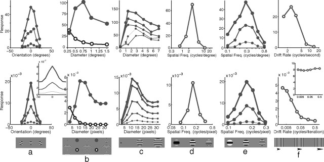
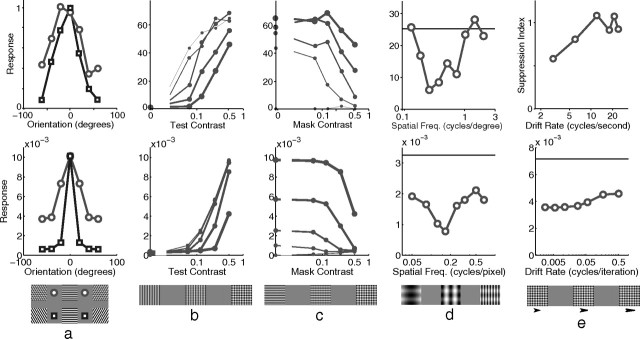
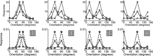
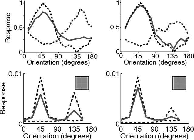
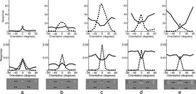
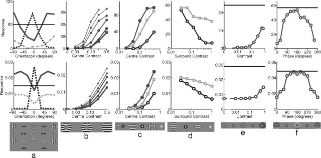
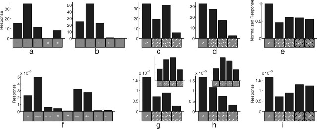
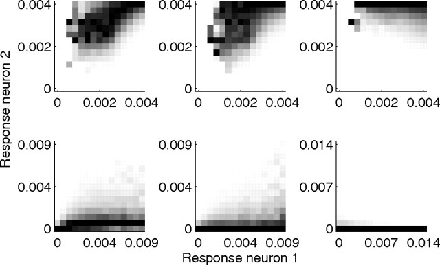
A simple model is shown to account for a large range of V1 classical, and nonclassical, receptive field properties including orientation tuning, spatial and temporal frequency tuning, cross-orientation suppression, surround suppression, and facilitation and inhibition by flankers and textured surrounds. The model is an implementation of the predictive coding theory of cortical function and thus provides a single computational explanation for a diverse range of neurophysiological findings. Furthermore, since predictive coding can be related to the biased competition theory and is a specific example of more general theories of hierarchical perceptual inference, the current results relate V1 response properties to a wider, more unified, framework for understanding cortical function.


Figures

Figure 1.
Figure 1.
The PC/BC model: a reformulation of predictive coding (Rao and Ballard, 1999) that can be interpreted as a form of biased competition model. The rectangles represent populations of neurons, with y labeling populations of prediction neurons and e labeling populations of error-detecting neurons. The open arrows signify excitatory connections, the filled arrows indicate inhibitory connections, the crossed connections signify a many-to-many connectivity pattern between the neurons in two populations, the parallel connections indicate a one-to-one mapping between the neurons in two populations, and the large shaded boxes with rounded corners indicate different cortical areas or processing stages.
Figure 2.
Figure 2.
The model of V1 implemented using PC/BC. The prediction neurons (labeled y) are assumed to correspond to V1 simple cells and the response of one of these neurons is recorded. The RFs of these prediction neurons are determined by the definition of the weight matrix W. Prediction neurons compete to represent the input stimulus x via divisive feedback, which acts on the error-detecting neurons (labeled e) and is carried by connections from the prediction neurons to the error-detecting neurons, which have strength proportional to the corresponding reciprocal weights from the error-detecting neurons to the prediction neurons.
Figure 3.
Figure 3.
The synaptic weights used in the PC/BC model of V1. a, A family of 32 Gabor functions (8 orientation and 4 phases) used to define the RFs of the neurons in the model. b, The actual synaptic weights of the model neurons were created by separating the positive and negative parts of the Gabor function into separate (non-negative) ON and OFF weights (shown for the bottom right Gabor function only). Each Gabor kernel is 21 × 21 pixels, and hence each prediction neuron in the model receives 21 × 21 × 2 = 882 synaptic weights.
Figure 4.
Figure 4.
The PC/BC model of V1 implemented using convolution and with separate ON and OFF channels. The input image I is preprocessed by convolution with a circular-symmetric on-center/off-surround kernel (to generate the input to the ON channel of the V1 model) and a circular-symmetric off-center/on-surround kernel (to generate the input to the OFF channel of the V1 model). The prediction neurons (labeled Y), which represent V1 simple cells, generate the responses that were recorded during the experiments. These responses were generated by convolving the outputs of the (ON and OFF channels of the) error-detecting neurons (labeled E) with (the ON and OFF channels of) a number of kernels representing V1 RFs. This convolution process effectively reproduces the same RFs at every pixel location in the image. The responses of the error-detecting neurons are influenced by divisive feedback from the prediction neurons, which is also calculated by convolving the prediction neuron outputs with the weight kernels.
Figure 5.
Figure 5.
Basic tuning properties. The top row shows neurophysiological data from representative single cells in V1, and the bottom row shows corresponding simulation results. a, Response as a function of grating orientation relative to the preferred orientation of the neuron. Neurophysiological data for a simple cell in cat V1 [adapted from Skottun et al. (1987), their Fig. 3a]. The thickness of each line corresponds to the contrast of the stimulus used as follows: 5% (thin), 20% (medium), and 80% (thick). The inset to the simulation data shows the response of the model without competition, created by recording the linear response generated at the first iteration of the algorithm (see Materials and Methods). b, Response as a function of the diameter of a circular grating (filled circles) and as a function of the inner diameter of an annular grating (open circles). Neurophysiological data for a cell in primate V1 [adapted from Jones et al. (2001), their Fig. 1]. c, Response as a function of grating diameter with variable grating contrast. Shown are neurophysiological data for a cell in primate V1 [adapted from Cavanaugh et al. (2002a), their Fig. 8]. The thickness of each line corresponds to the contrast of the stimulus used as follows: 6% (thinnest), 13, 25, 50, and 100% (thickest). d, Response as a function of grating spatial frequency. Shown are neurophysiological data for a cell in primate V1 [adapted from Webb et al. (2005), their Fig. 2a]. e, Response as a function of grating spatial frequency with variable grating contrast. Shown are neurophysiological data for a simple cell in cat V1 [adapted from Skottun et al. (1987), their Fig. 4a]. The thickness of each line corresponds to the contrast of the stimulus used as follows: 5% (thin), 20% (medium), and 80% (thick). f, Response as a function of grating temporal frequency. Shown are neurophysiological data for a cell in cat V1 [adapted from Freeman et al. (2002), their Fig. 3c]. The inset to the simulation data shows the response summed over all neurons within 11 pixels of the neuron recorded in the main figure.
Figure 6.
Figure 6.
Cross-orientation suppression. The top row shows neurophysiological data from representative single cells in V1, and the bottom row shows corresponding simulation results. a, Response as a function of the orientation of a single grating (squares) and as a function of the orientation of a mask grating additively superimposed on an optimally orientated grating (circles). Shown are neurophysiological data for a cell in cat V1 [data from Bonds (1989); figure adapted from Schwartz and Simoncelli (2001), their Fig. 5]. b, Response as a function of the contrast of the optimally orientated grating for several different orthogonal mask contrasts. The thickness of each line corresponds to the contrast of the mask grating as follows: 0% (thinnest), 6, 12, 25, and 50% (thickest). Shown are neurophysiological data for a cell in cat V1 [adapted from Freeman et al. (2002), their Fig. 2]. c, The data in b replotted to show response as a function of the contrast of the orthogonal mask grating for several different optimally oriented grating contrasts. The thickness of each line corresponds to the contrast of the optimally oriented grating as follows: 0% (thinnest), 6, 12, 25, and 50% (thickest). d, Response as a function of the spatial frequency of an orthogonal mask grating. Shown are neurophysiological data for a simple cell in cat V1 [adapted from DeAngelis et al. (1992), their Fig. 3b]. The horizontal lines show the response to the optimally oriented grating presented in isolation. e, Response as a function of the temporal frequency of an orthogonal mask grating. Shown are neurophysiological data for a cell in cat V1 [adapted from Freeman et al. (2002), their Fig. 3e]. Note that the physiological data are presented in the form of a suppression index: a value of 0 corresponds to no suppression and values >0 correspond to stronger suppression. For the model data, the horizontal line shows the response to the optimally orientated gating in the absence of the mask; hence the mask generates strong suppression across a range of temporal frequencies, consistent with the neurophysiological data.
Figure 7.
Figure 7.
Cross-orientation suppression with varying orientation. Response as a function of grating orientation for two gratings presented in isolation (dashed lines) and for both gratings presented simultaneously (solid lines). The top row shows responses from a single cell in tree shrew V1 [adapted from MacEvoy et al. (2009), their Fig. 4], and the bottom row shows responses from the model. The angle between the two gratings increases from left to right: 22.5° (left column), 45, 67.5, and 90° (right column).
Figure 8.
Figure 8.
Cross-orientation suppression with varying orientation and contrast. Response as a function of grating orientation for two gratings presented in isolation (dashed lines) and for both gratings presented simultaneously (solid lines). The top row shows population responses measured using intrinsic signal optical imaging in tree shrew V1 [adapted from MacEvoy et al. (2009), their Fig. 3], and the bottom row shows responses from a single neuron in the model. The angle between the two gratings was 90°. One grating was presented at a lower contrast than the other: for the left column, the contrasts were 0.5 and 0.25, and for the right column, the contrasts were 0.5 and 0.125.
Figure 9.
Figure 9.
Surround suppression with variable surround orientation. The top row shows neurophysiological data from representative single cells in primate V1 [adapted from Jones et al. (2002), their Fig. 1], and the bottom row shows corresponding simulation results. a–e, Each column shows a different pattern of behavior identified by Jones et al. (2002) as follows: orientation contrast suppression (a), non-orientation-specific suppression (b), mixed general suppression (c), orientation alignment suppression (d), and orientation contrast facilitation (e). In each case, response is plotted as a function of grating orientation relative to the preferred orientation of the neuron for a central grating presented in isolation (dashed lines) and as a function of the orientation of a surrounding annulus in the presence of an optimally oriented central grating (solid lines). Note that for the neurophysiological data in a, but not the other plots, only the response at 0° is shown for the condition in which the center is presented in isolation (circular marker). The results for the model were generated using a center diameter of the following: 7 pixels (a), 11 pixels (b), 13 pixels (c), 17 pixels (d), and 19 pixels (e). The inner diameter of the surrounding annulus was equal to the center diameter in each case.
Figure 10.
Figure 10.
Surround suppression with variable contrast and variable surround phase. The top row shows neurophysiological data from representative single cells in V1, and the bottom row shows corresponding simulation results. a, Response plotted as a function of grating orientation relative to the preferred orientation of the neuron for a central grating presented in isolation (dashed line), as a function of the orientation of a surrounding annulus in the presence of an optimally oriented central grating (solid line), and as a function of surround orientation for a center contrast much smaller than the surround contrast (dash-dot line). The horizontal lines show the response to the low-contrast center stimulus presented alone at the preferred orientation. Shown are neurophysiological data for a cell in primate V1 [adapted from Levitt and Lund (1997), their Fig. 1d]. b, Response as a function of the contrast of the central grating in the presence of an iso-oriented surround. Shown are neurophysiological data for a cell in primate V1 [adapted from Cavanaugh et al. (2002a), their Fig. 5b]. The thickness of each line corresponds to the contrast of the grating in the annular surround: 0% (thinnest), 3, 6, 12, 25, and 50% (thickest). c, Response as a function of the contrast of the central grating with no surround (filled circles), an iso-oriented surround (open circles), and an orthogonal surround (squares); in the latter two cases, the surround contrast was fixed at 50%. Shown are neurophysiological data for a simple cell in primate V1 [adapted from Cavanaugh et al. (2002b), their Fig. 5a]. d, Response as a function of the contrast of the surround grating with an iso-oriented surround (circles), and an orthogonal surround (squares); in both cases, the center contrast was fixed at 40%. Shown are neurophysiological data for a cell in primate V1 [adapted from Webb et al. (2005), their Fig. 6]. e, Response as a function of the contrast of an orthogonal surround grating superimposed on an iso-oriented surround grating in the presence of an optimally oriented center. Shown are neurophysiological data for a cell in cat V1 [adapted from Walker et al. (2002), their Fig. 2b]. The contrast of the center and the iso-oriented surround were fixed at 30%. The horizontal lines indicate the response to the central grating in isolation. f, Response as a function of the phase of the grating in the surround. Shown are neurophysiological data for a cell in primate V1 [adapted from Xu et al. (2005), their Fig. 2a]. The horizontal lines indicate the response to the central grating in isolation.
Figure 11.
Figure 11.
The effect of flankers and textured surrounds on neural response. a, Response to one set of flanker configurations of a single cell in primate V1 [adapted from Kapadia et al. (2000), their Fig. 7a]. b, Response to a second set of flanker configurations of a different cell in primate V1 [adapted from Kapadia et al. (1995), their Fig. 11a]. c, Average response of 28 cells in primate V1 that were classified as orientation contrast cells [adapted from Nothdurft et al. (1999), their Fig. 4a]. d, Average response of 14 cells in primate V1 that were classified as uniform cells [adapted from Nothdurft et al. (1999), their Fig. 4b]. e, Average response of 124 cells in primate V1 to textured surrounds with varying contrast [adapted from van der Smagt et al. (2005), their Fig. 4a]. f, Response of a model neuron to both sets of flanker configurations shown in a and b. g, Response of a model neuron to texture patterns like those in c and d, in which the spacing between bars was 1.6 times the bar length. h, Response of a model neuron to similar texture patterns created using a spacing of two times the bar length. The insets to g and h show the linear response of the model for the two different texture spacings. i, Response of a model neuron to texture patterns with varying contrast, as used in e. Note: The icons used to represent the stimulus configurations in c–e and g–i show only the central portion of the actual images used in the experiments.
Figure 12.
Figure 12.
Conditional probability histograms of responses to a natural image. In each histogram, a column indicates the probability that neuron 2 generates an output of the given magnitude given that neuron 1 has generated an output of the magnitude shown on the abscissa. A dark pixel indicates a high conditional probability. Each column in each histogram has been independently rescaled to fill the full range of intensity values. The top row shows histograms for the initial linear response of the model (without competition). The bottom row shows histograms for the model including inhibition. Histograms in the left-hand column are for two neurons tuned to the same orientation but 2 pixels apart, so that RFs are parallel. Histograms in the middle column are for two neurons tuned to the same orientation but 6 pixels apart, so that RFs are parallel. Histograms in the right-hand column are for two neurons tuned to orthogonal directions at the same location. It can be seen that, without competition, the responses are correlated such that the higher the response at the first neuron, the higher the response is likely to be from the second neuron. It is also the case that all neurons tend to generate strong responses. After competition has occurred, the responses are much more sparse (fewer neurons generate strong responses), and the dependency between different neurons is substantially reduced, and for neurons at the same location (bottom-right histogram) the correlation is eliminated. The image used to generate these histograms was image number 23 from the still image database used in the study by van Hateren and van der Schaaf (1998).

Similar articles

Cited by

References

    1. Adorján P, Levitt JB, Lund JS, Obermayer K. A model for the intracortical origin of orientation preference and tuning in macaque striate cortex. Vis Neurosci. 1999;16:303–318. - PubMed
    1. Albrecht DG, Geisler WS. Motion selectivity and the contrast-response function of simple cells in the visual cortex. Vis Neurosci. 1991;7:531–546. - PubMed
    1. Angelucci A, Bullier J. Reaching beyond the classical receptive field of V1 neurons: horizontal or feedback axons? J Physiol Paris. 2003;97:141–154. - PubMed
    1. Angelucci A, Levitt JB, Walton EJ, Hupe JM, Bullier J, Lund JS. Circuits for local and global signal integration in primary visual cortex. J Neurosci. 2002;22:8633–8646. - PMC - PubMed
    1. Barlow HB. What is the computational goal of the neocortex? In: Koch C, Davis JL, editors. Large-scale neuronal theories of the brain. Cambridge, MA: MIT; 1994. pp. 1–22. Chap 1.

Publication types

MeSH terms

LinkOut - more resources