Columnar connectivity and laminar processing in cat primary auditory cortex

Abstract

Background: Radial intra- and interlaminar connections form a basic microcircuit in primary auditory cortex (AI) that extracts acoustic information and distributes it to cortical and subcortical networks. Though the structure of this microcircuit is known, we do not know how the functional connectivity between layers relates to laminar processing.

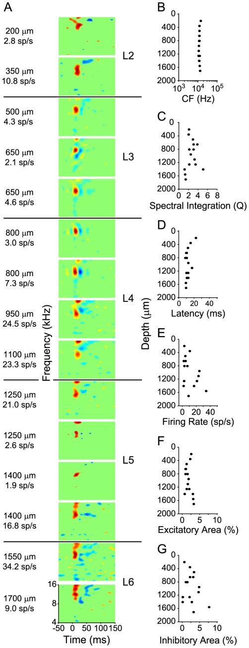
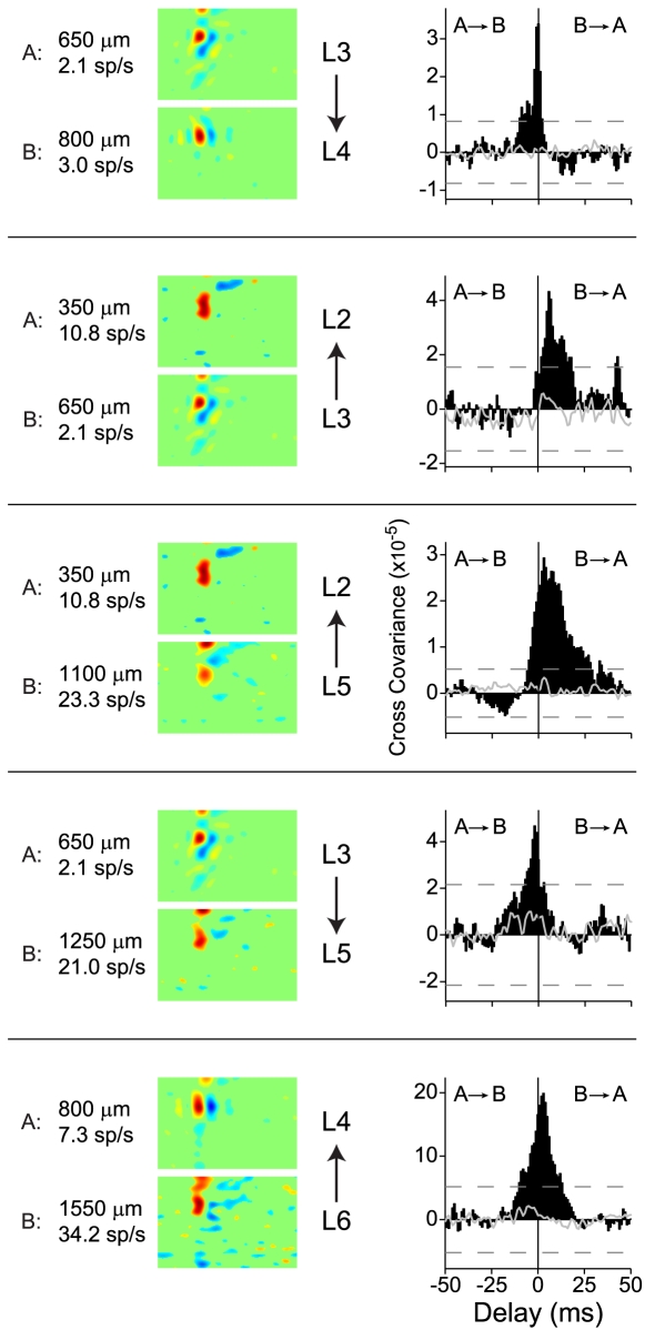
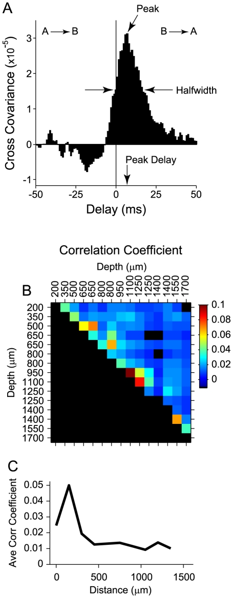
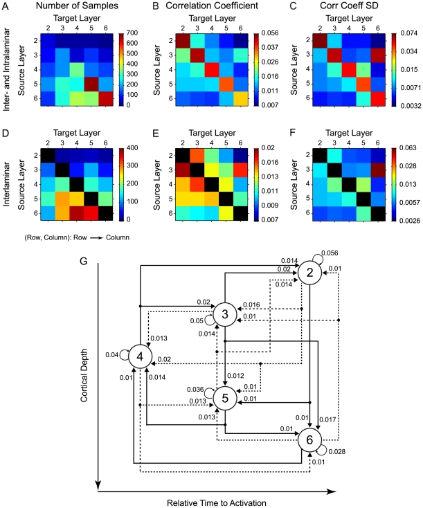
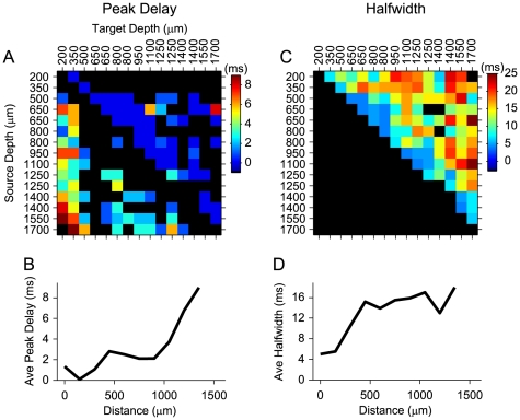
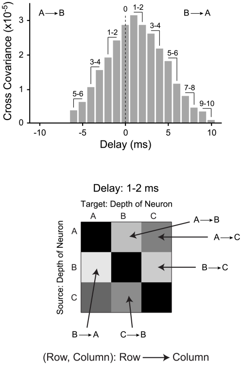
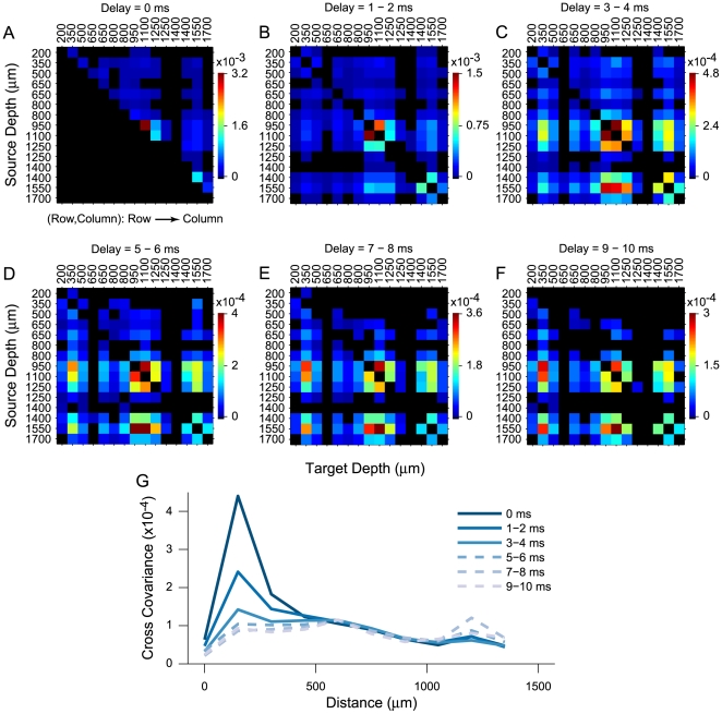
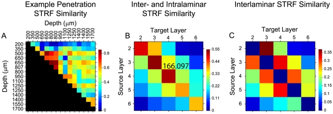
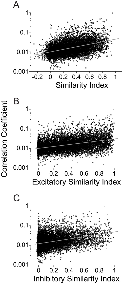
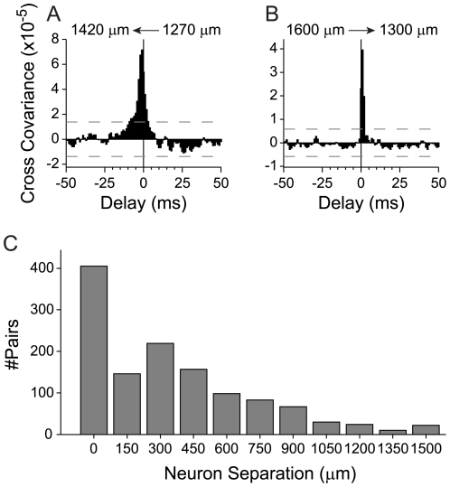
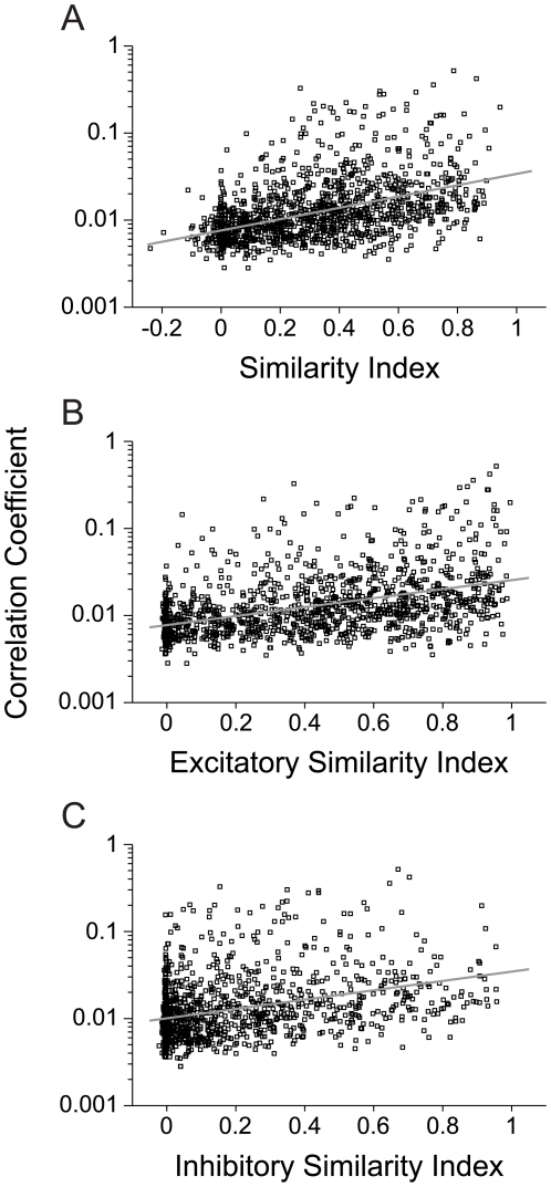
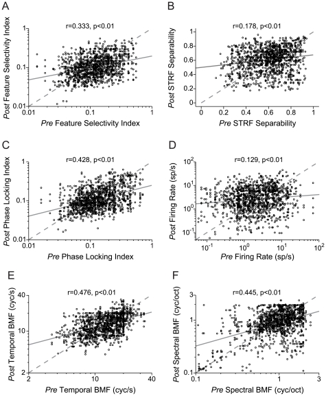
Methodology/principal findings: We studied the relationships between functional connectivity and receptive field properties in this columnar microcircuit by simultaneously recording from single neurons in cat AI in response to broadband dynamic moving ripple stimuli. We used spectrotemporal receptive fields (STRFs) to estimate the relationship between receptive field parameters and the functional connectivity between pairs of neurons. Interlaminar connectivity obtained through cross-covariance analysis reflected a consistent pattern of information flow from thalamic input layers to cortical output layers. Connection strength and STRF similarity were greatest for intralaminar neuron pairs and in supragranular layers and weaker for interlaminar projections. Interlaminar connection strength co-varied with several STRF parameters: feature selectivity, phase locking to the stimulus envelope, best temporal modulation frequency, and best spectral modulation frequency. Connectivity properties and receptive field relationships differed for vertical and horizontal connections.

Conclusions/significance: Thus, the mode of local processing in supragranular layers differs from that in infragranular layers. Therefore, specific connectivity patterns in the auditory cortex shape the flow of information and constrain how spectrotemporal processing transformations progress in the canonical columnar auditory microcircuit.

Figure 1. Example multi-channel recording, with spectrotemporal receptive fields (STRFs) and response parameters.

(A) STRFs from simultaneously recorded columnar neurons in AI. Each row represents a single neuron. The cortical depth and firing rate of each neuron are indicated to the left of the STRFs. STRFs with the same depth values indicate that multiple neurons were recorded from the same electrode channel. (B) Characteristic frequency (CF) from the excitatory subfield of the STRFs. (C) Spectral integration, or quality factor (Q), of the excitatory subfield of the STRFs. (D) Peak excitatory latency in the STRFs. (E) Firing rate over the ripple stimulus duration. (F) STRF excitatory area percentage, or proportion of pixels, in the STRFs that were excitatory. (G) STRF inhibitory area percentage. Excitatory and inhibitory area percentages were determined by dividing the number of excitatory or inhibitory pixels by the total number of STRF pixels.

Figure 2. Example STRFs and temporal interactions between neurons in an AI column.

Data are from the example penetration shown in Fig. 1. Each row represents a separate pair of neurons. (Left) Depth, firing rate, and STRF of the neurons for which cross-covariance functions were computed. Layer assignments are to the right of the STRFs (L2-L6). (Right) Cross-covariance functions for the pairs of neurons in the left column. Arrows indicate direction of the temporal interaction: negative delays mean A fired before B, positive delays mean B fired before A. Dashed lines indicate 99% confidence intervals. Gray curves indicate shift predictors, i.e., the timing distribution of non-simultaneously recorded spike trains. The laminar connection patterns most consistent which the cross-covariance function are shown to the right of the each STRF pair.

Figure 3. Analysis of cross-covariance functions.

(A) Peak value, delay at which the peak occurs, and cross-covariance function halfwidth were extracted from each cross-covariance function. Peak delay and halfwidth are calculated with respect to the maximum (Peak) in the function. (B) Correlation coefficient depth matrix, calculated from cross-covariance functions for the data in Fig. 1. Since the matrix is symmetric, values below the diagonal are not shown. Black squares above the diagonal indicate non-significant connections. Duplicated depth values represent neurons recorded at the same depth. (C) Correlation coefficient versus distance between neurons for the data in (B).

Figure 4. Summary of AI interlaminar connection strengths.

For each neuron pair with a significant correlation we determined the direction of the connection and the correlation coefficient, or connection strength. (A) Number of pairs for all inter- and intralaminar data, grouped by laminar connection pattern. Each element in the matrix is in Row to Column form (Row, Column), which implies that the connection was from Row ( =  source layer) to Column ( =  target layer). The parameter value is indicated by the color. Element (4,3) implies the number of significant connections from layer 4 to layer 3 in our dataset. (B) Mean inter- and intralaminar connection strength, or correlation coefficient, for all significantly connected neuron pairs. (D, E) same as (A,B), with the intralaminar contributions removed to emphasize patterns of inter-laminar connections. (D) Number of connected pairs for each interlaminar combination. (E) Mean inter-laminar connection strength. (C, F) Standard deviation (SD) of inter- and intralaminar connection strength distributions, corresponding to the data in (B,E). (G) Layer connectivity diagram for the data in (B). Interlaminar and interlaminar connections are shown. Solid lines indicate feedforward connections in the auditory cortical microcircuit. Dashed lines indicate feedback connections. Values indicate the connection strengths from (B). Layers, indicated by circles, are vertically arranged to coincide with cortical depth. Layers are also organized horizontally to indicate the relative response time of each layer, as determined from latency analysis .

Figure 5. Example temporal interaction parameter matrices for neurons in an AI column.

Data from example penetration in Fig. 1. Matrix values are indexed according to specific neuron combinations indicated by the depths listed above and to the left of the plots in (A, C). (A) Peak delays from cross-covariance functions. Absolute values of peak delays are shown. Each element in the matrix is in Row to Column form, (Row, Column), which implies that the connection was from Row to Column. The signs (+ or −) of peak delays were used to determine the direction of the connection. Black matrix elements indicate non-significant connections or connections not consistent with cross-covariance functions. (B) Average peak delay as a function of intra-columnar distance between neurons for the data in (A). (C) Halfwidths of cross-covariance functions. Values below the diagonal are not shown since the matrix is symmetric. Black matrix elements above the diagonal indicate non-significant connections. (D) Average halfwidth versus intra-columnar distance between neurons for the data in (C).

Figure 6. Temporal interaction parameters as a function distance between neurons.

(A) Population data for peak delay versus neuron separation. Cross-covariance function peak delay increases with increasing cortical distance between functionally connected neurons. Data are mean +/− S.E.M. (B) Population data for halfwidth versus neuron separation. Halfwidth increases with neuron separation. Data are mean +/− S.E.M. (C) Frequency histogram of neuron separation for functionally connected neurons.

Figure 7. Method for obtaining values for Synchronization Matrices (SMs).

(Top) Example cross-covariance function. Values for SMs are obtained by averaging cross-covariance function values at different spiking delays (1 and 2, 3 and 4, 5 and 6, 7 and 8, and 9 and 10 ms delays). The same procedure is used for negative delays. Only significant cross-covariance function values are shown. Non-significant values (−7 to −10) are excluded. (Bottom) Example SM for a delay of 1–2 ms for 3 neurons in a penetration. Each element in the SM represents a connection strength and connection direction. Elements are ordered so element (Row, Column) in the matrix indicates cross-covariance function values consistent with a Row (source layer) to Column (target layer) connection.

Figure 8. Synchronization Matrices (SMs) for neurons in an AI column.

Data from example penetration in Figure 1. (A–F) SMs. Each pixel in an SM represents the strength of the cross-covariance function between the neurons whose positions are listed above and to the left of the plot (blue to red indicates increasing connection strength). Matrices are ordered so that element (A,B), or (Row, Column), represents the cross-covariance function value consistent with an A to B flow of information. The SM values are obtained by averaging the cross-covariance function values at the delays listed above each plot. The strength of neural synchronization between local neurons decreases for longer delays but stays the same or slightly increases between more distant neuron pairs (increasing SM values at off-diagonal positions). Black pixels indicate cross-covariance function values that did not achieve significance. (G) Cross-covariance function values versus distance between neurons at multiple delays. Data are obtained from the SMs in (A–F).

Figure 9. STRF similarity for functionally connected neurons.

(A) Example STRF similarity index matrix for the neurons in Fig. 1. Each matrix element represents the similarity between the STRFs of different neurons. The similarity between STRFs is greatest between neurons at supragranular (200–800 µm) and granular (800–1100 µm) layer depths. Data below the diagonal are not shown since the matrix is symmetric. (B) Intra- and interlaminar STRF similarity across all data, grouped according to layer. STRFs are most similar for connected neurons within the same layer. (C) Interlaminar STRF similarity data (data from (B) with intralaminar data removed).

Figure 10. Connection strength versus STRF similarity.

Correlation coefficient values as a function of (A) Full STRF similarity between functionally connected neurons (r = 0.464, p<0.01, t-test). (B) Similarity between only the excitatory STRF subfields (r = 0.433, p<0.01, t-test). (C) Only the inhibitory STRF subfields (r = 0.379, p<0.01, t-test). (N = 8364).

Figure 11. Putative monosynaptically connected neurons.

Connections were classified as monosynaptic if peak delays were 1–4 ms, and if cross-covariance function halfwidths were less than 10 ms. (A,B) Examples cross-covariance functions for two putative monosynaptically connected neurons. (A) Functional connection between two cells in layer 5. The direction of the connection is from the cell at 1270 µm to the cell at 1420 µm. (B) Functional connection from a cell in layer 6 (1600 µm) to a cell in layer 5 (1300 µm). (C) Vertical distance between neurons for all monosynaptic connections (N = 1203 pairs).

Figure 12. Correlation coefficient versus STRF similarity for monosynaptic functionally connected neurons (N = 1203 pairs).

STRF similarity was computed for (A) the full STRF (r = 0.444, p<0.01, t-test), (B) the excitatory subfields of the STRF (r = 0.434, p<0.01, t-test), and (C) the inhibitory subfields of the STRF (r = 0.348, p<0.01, t-test).

Figure 13. Comparison of receptive field parameters for monosynaptic functionally connected neurons (N = 1203 pairs).

Each data point represents a connected pair. The abscissa (Pre) represents the parameter value for the neuron in the pair that responded first, or was Presynaptic, according to the peak delay in the cross-covariance function. The ordinate (Post) represents the neuron whose response came after the other neuron in the pair, or was Postsynaptic. (A) Feature Selectivity Index (r = 0.333, p<0.01). (B) STRF Separability (r = 0.178, p<0.01). (C) Phase Locking Index (r = 0.428, p<0.01). (D) Firing Rate (r = 0.129, p<0.01). (E) Temporal Best Modulation Frequency (r = 0.476, p<0.01). (F) Spectral Best Modulation Frequency (r = 0.445, p<0.01; t-test used for all comparisons).

References

1. Phillips DP, Irvine DR. Responses of single neurons in physiologically defined primary auditory cortex (AI) of the cat: frequency tuning and responses to intensity. J Neurophysiol. 1981;45:48–58. - PubMed
1. Szymanski FD, Garcia-Lazaro JA, Schnupp JW. Current source density profiles of stimulus-specific adaptation in rat auditory cortex. J Neurophysiol. 2009;102:1483–1490. - PubMed
1. Kaur S, Rose HJ, Lazar R, Liang K, Metherate R. Spectral integration in primary auditory cortex: laminar processing of afferent input, in vivo and in vitro. Neuroscience. 2005;134:1033–1045. - PubMed
1. Wallace MN, Palmer AR. Laminar differences in the response properties of cells in the primary auditory cortex. Exp Brain Res. 2008;184:179–191. - PubMed
1. Lee CC, Winer JA. Connections of cat auditory cortex: I. Thalamocortical system. J Comp Neurol. 2008;507:1879–1900. - PMC - PubMed
Publication types