

Review
doi: 10.1021/cr900396q.
Theory, instrumentation, and applications of electron paramagnetic resonance oximetry
Affiliations
- PMID: 20218670
- PMCID: PMC2868962
- DOI: 10.1021/cr900396q
Item in Clipboard
Review
Theory, instrumentation, and applications of electron paramagnetic resonance oximetry
Chem Rev.
.
No abstract available
Figures
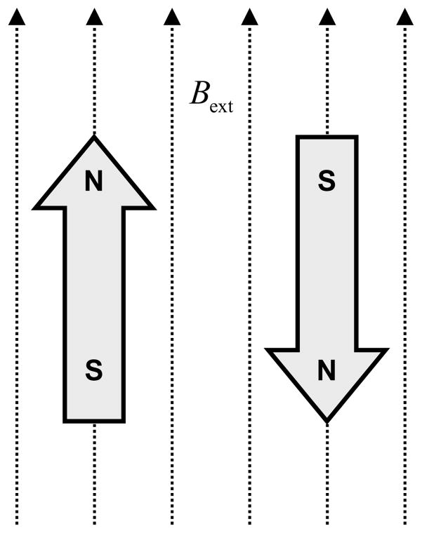
Lowest (left) and highest (right) energy orientations of the magnetic moment of an unpaired electron in the presence of an external magnetic field Bext.
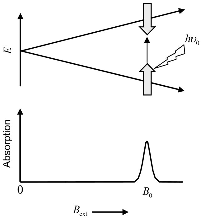
Zeeman splitting in the presence of an external magnetic field Bext (neglecting second order effects like hyperfine splitting).
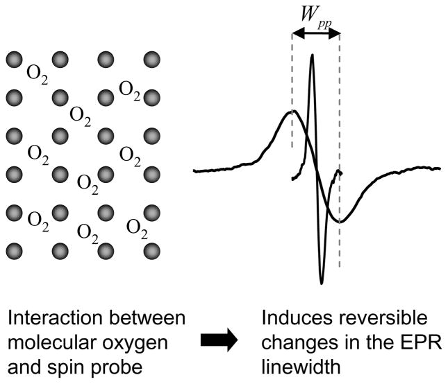
Effect of oxygen on exchange narrowed lineshape. Black dots represents spin probe molecules. Introduction of O2 induces line broadening measured by peak-to-peak linewidth Wpp.
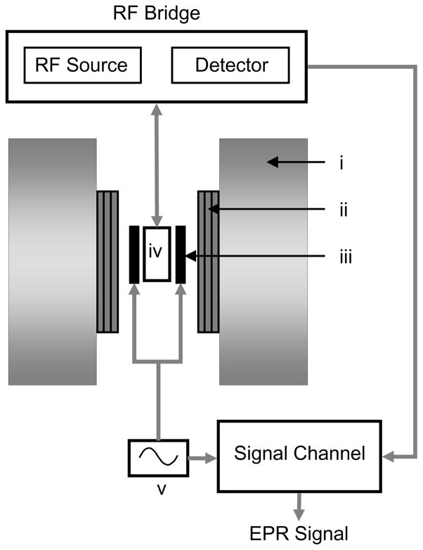
A basic layout of a CW EPR spectrometer and imager. i, main magnet; ii, gradient coil assembly; iii, field modulation coil; iv, resonator; v, field modulation source.
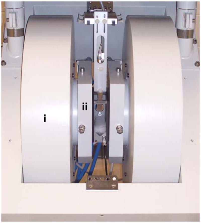
Bruker (Bruker BioSpin, Billerica, MA, USA) L-band EPR imager. Main magnet (i) and magnetic field gradient assembly (ii).
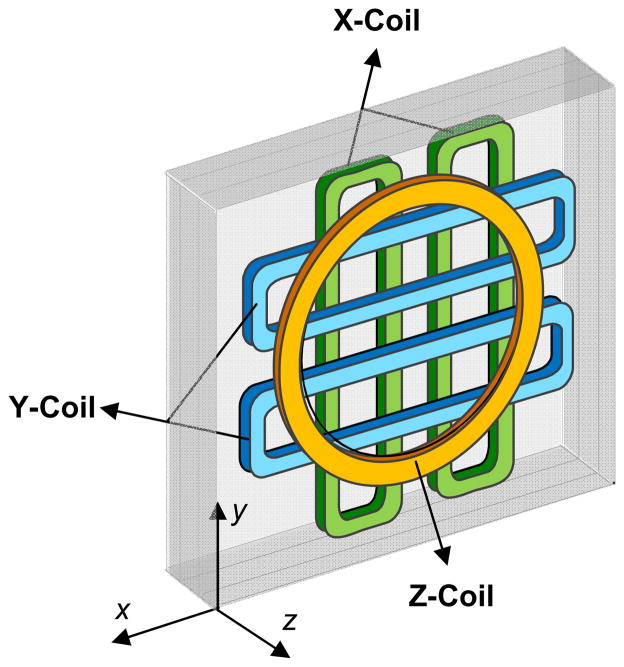
Gradient coil assembly. Left-side enclosure of a 3D gradient coil assembly is shown. The Z-gradient is generated using Maxwell coils, while X- and Y-gradients are generated using flat pair coils.
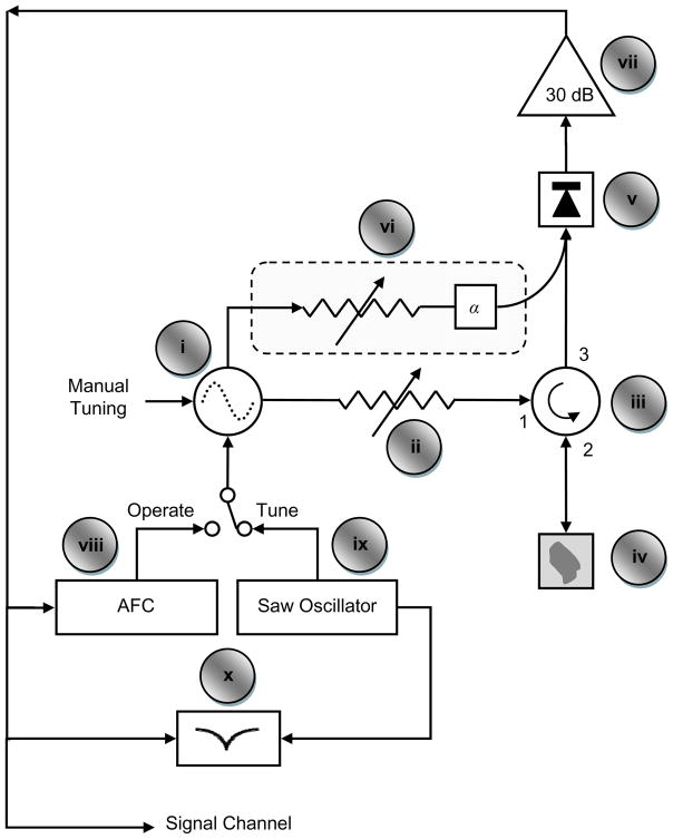
Layout of a typical CW EPR bridge. Adapted with permission from Mr. Eric Kesselring.
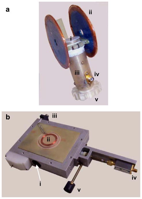
Two frequently used resonator designs for EPR spectrometer. a: Surface bridged, loop-gap resonator (LGR). The LGR resonator structure is housed inside a metallic tubular shield. Legends: i, active surface area for sample; ii, filed modulation coils; iii, resonator shield; iv, RF input connector; v, coupling adjustment ring. The connector for field modulation coil is not visible from this view. The resonant frequency of this unloaded LGR was 1.25 GHz. b: Volume reentrant resonator (RER). The RER houses a cylindrical cavity of 24 mm diameter and 22 mm of effective length. Legends: i, sample cavity opening; ii, modulation coils; iii, connector of modulation coils; iv, RF input connector; v, coupling adjustment knob. The resonant frequency of this unloaded RER was 1.27 GHz
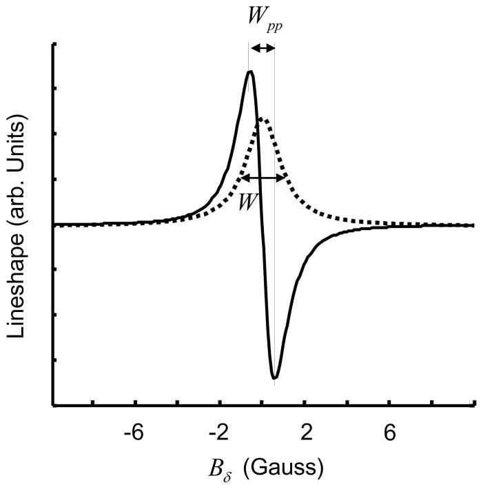
Lorentzian lineshape (dotted line) with FWHM linewidth W = 1 G. First derivative Lorentzian lineshape (solid line) with peak-to-peak linewidth Wpp =0.58 G. For a Lorentzian lineshape,
.
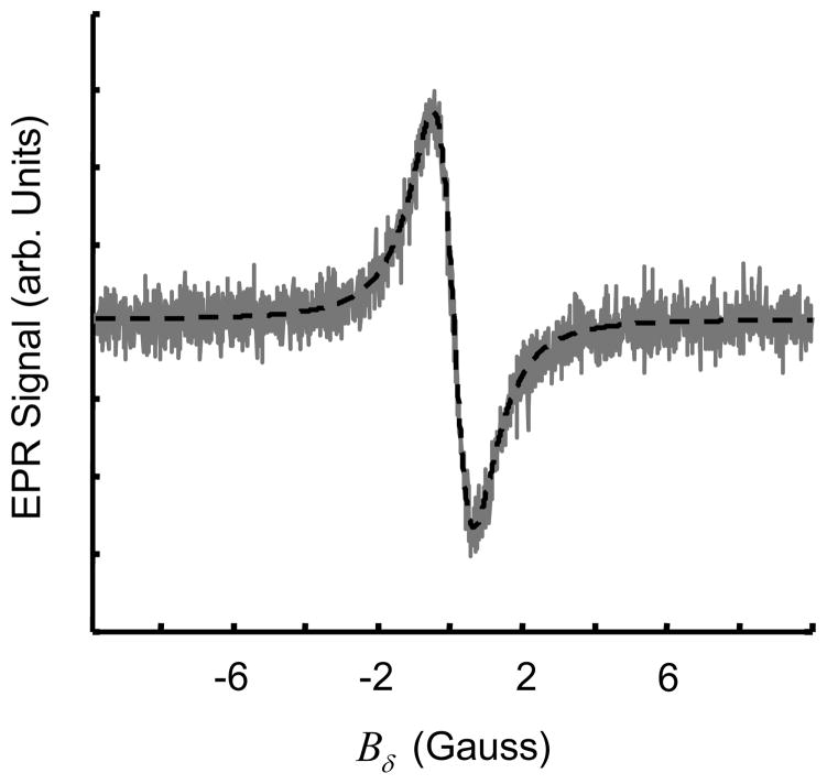
Measured data (gray line) is generally noisy and curve fitting (dashed line) is applied to extract the linewidth information.
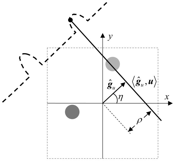
Projection acquisition for a 2D spatial digital object. Angle η defines orientation of the applied gradient gu, ρ defines the distance of resonant plane 〈ĝu,u〉 from the origin.
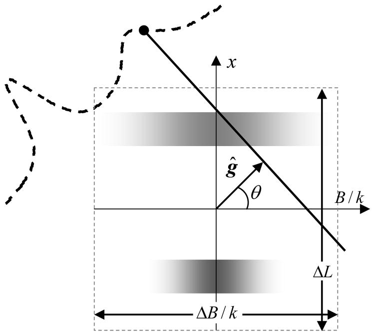
Data collection for a 2D spectral-spatial digital object. The vertical-axis represents the spatial dimension while the horizontal-axis represents the spectral dimension. The figure shows two regions; the one on the top has a large linewidth while on the bottom exhibits a smaller linewidth. Here, k = ΔB/ΔL and ĝ = (ĝu sinθ,cosθ)is a generalized gradient vector which incorporates gradient strength with gradient orientation.
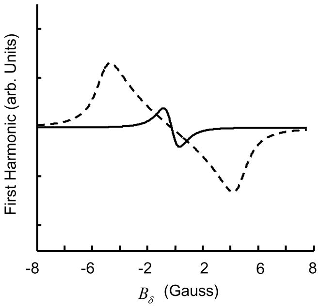
Effect of modulation amplitude Bm on lineshape. The solid line represents lineshape for a modulation amplitude which is 10% of linewidth W, while the dashed line represents the lineshape for a modulation amplitude which is 250% of W.
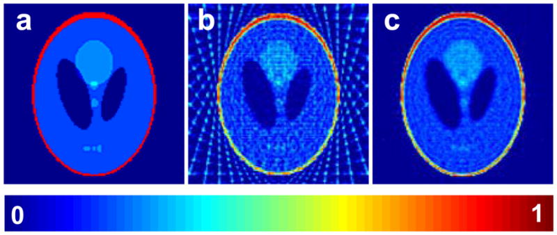
Comparison of an iterative reconstruction method with the commonly used filtered backprojection method. a: A 128×128 2D digital Shepp-Logan phantom; b: Reconstruction from filtered backprojection using 20 noiseless projections, after the reconstruction all pixels with negatives values were set to zero; c: Reconstruction based on algebraic reconstruction technique (ART) with nonnegativity constraint using 20 noiseless projections.
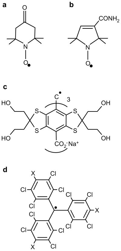
Chemical structure of soluble spin probes commonly used for EPR oximetry. a: Tempone (1-oxyl-2,2,6,6-tetramethyl-4-piperidione); b: CTPO (2,2,5,5-tetramethyl-3-pyrroline-1-oxyl-2-carboxamide); c: TAM (triarylmethyl) OX063; d: PTM (perchlorotriphenylmethyl) for X=Cl, PTM-TE for X= COOR, and PTM-TC for X=COOH;
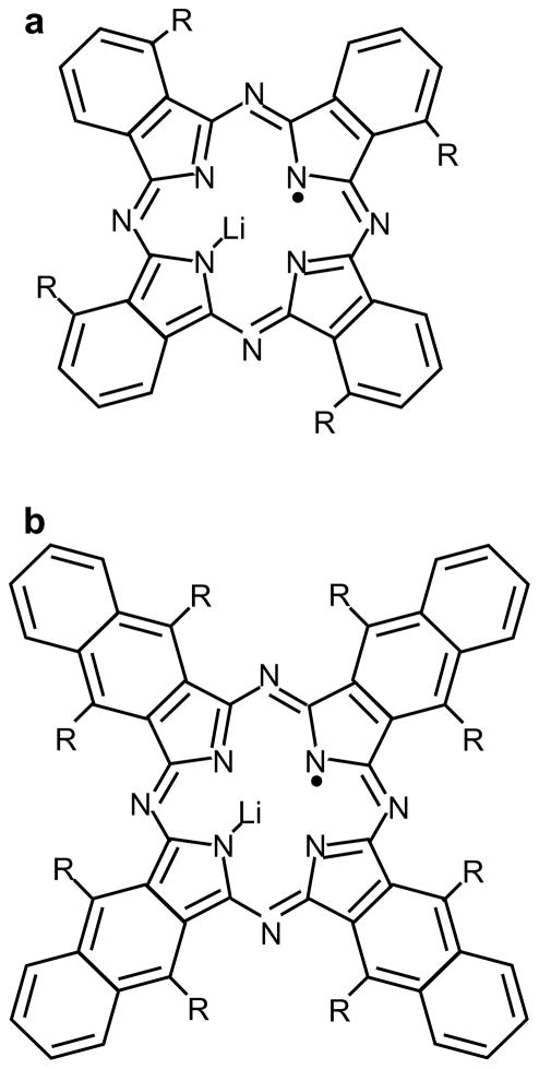
Chemical structure of particulate spin probes commonly used for EPR oximetry. a: LiPC for R=H and LiPc-α-OPh for R=phenoxy; b: LiNc for R=H and LiNc-BuO for R=O(CH2)3CH3
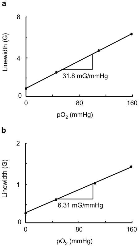
Effect of molecular oxygen on the EPR linewidth of LiNc (a) and LiNc-BuO (b) crystals. A linear variation of linewidth with the pO2 is observed for both the probes. For LiNc: anoxic linewith, 0.90 G; oxygen sensitivity, 31.8 mG/mmHg. For LiNc-BuO: anoxic linewidth=0.41 G; oxygen sensitivity=6.31 mG/mmHg. Measurements were conducted at L-band CW EPR spectrometer. The instrumental settings were: microwave power, 2 mW; modulation amplitude, 200 mG; modulation frequency, 100 kHz; receiver time constant, 10 ms; acquisition time, 10 s (single scan);
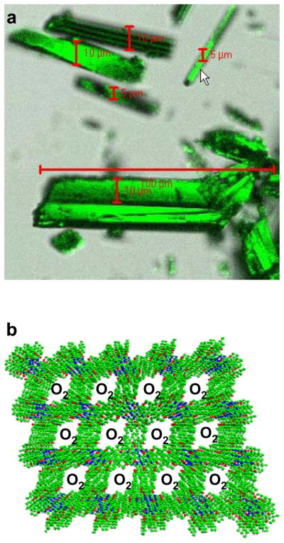
LiNc-BuO in crystalline form. a: Photograph of needle-shaped LiNc-BuO microcrystals; b: Stacking of LiNc-BuO molecules in a crystal. The EPR line-broadening occurs due to the diffusion of O2 into the microchannels and subsequent spin-spin interaction through the Heisenberg exchange mechanism. Image b is reprinted with permission from ref . Copyright 2006 The Royal Society of Chemistry. DOI: 10.1039/b517976a.
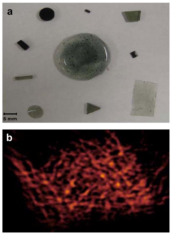
Chips fabricated by the encapsulation of LiNc-BuO particulates in PDMS. a: Pieces of polymerized LiNc-BuO with varying sizes, shapes and ratios of particulate to polymer. Dark shade indicates higher concentration of LiNc-BuO crystals. b: X-band EPR images of polymerized LiNc-BuO chip to evaluate spin distribution. Samples were imaged under anoxic conditions, in a sealed tube. Reprinted with permission from ref . Copyright 2009 Springer.
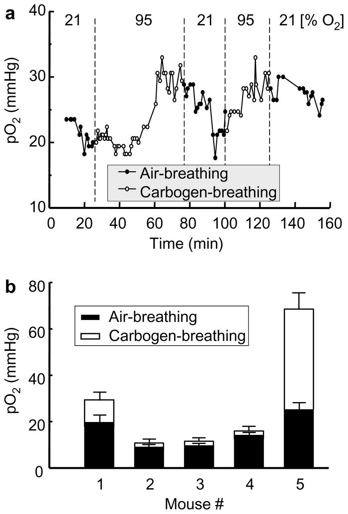
Effect of FiO2 (fraction of inspired oxygen) on the tumor pO2. Twenty μL of PTM-TE (12 mM in HFB) was injected directly into RIF-1 tumor grown in the hind leg of a C3H mouse. a: Change in pO2 in the tumor of a single animal while the FiO2 was successively switched between 21% and 95% (carbogen gas), as indicated. b: The pO2 values obtained before (FiO2 = 21%) and 20 min after changing the FiO2 to 95% in 5 different animals. Reprinted with permission from ref . Copyright 2007 Elsevier.
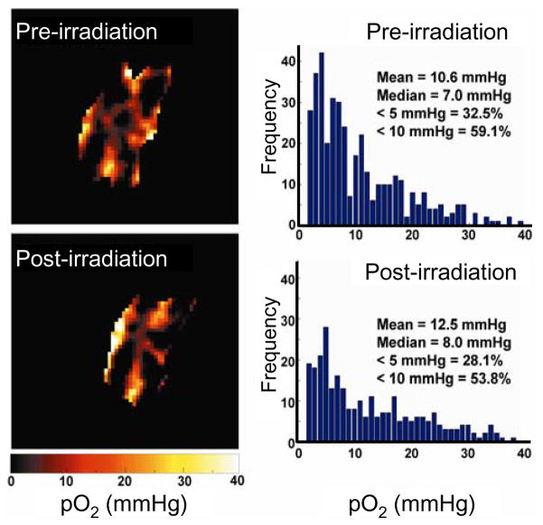
In vivo mapping of tumor pO2 during growth and after treatment with X-ray irradiation. Change and redistribution of tumor pO2 are shown for a small (volume 113 mm3) RIF-1 tumor before (pre-) and 1 h after (post-) X-ray irradiation. The tumor was implanted with RIF-1 cells internalized with nanoparticulates of LiNc-BuO. A dose of 30 Gy was delivered with 6-MeV electrons at a dose rate of 3 Gy/min. Redistribution is seen with a modest increase in the pO2. Reprinted with permission from ref . Copyright 2007 John Wiley and Sons.
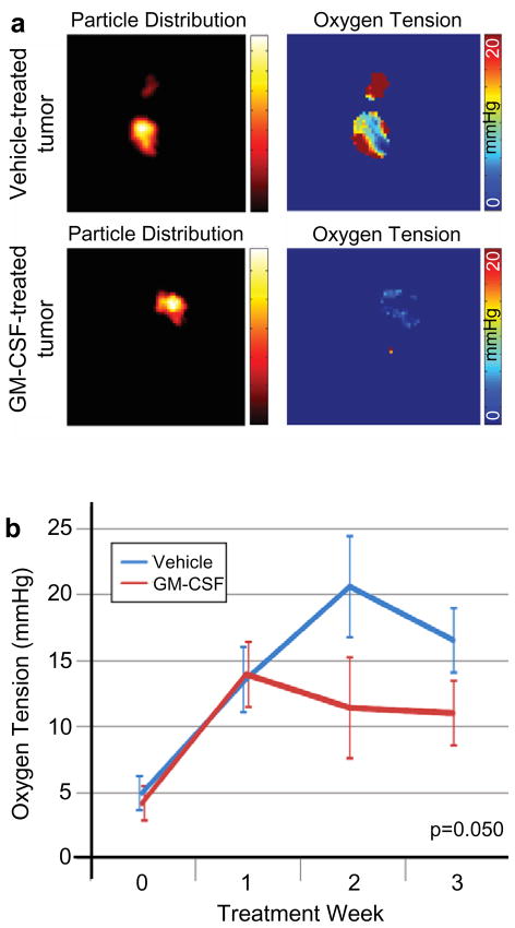
Intratumor GM-CSF treatment reduces oxygen levels within mammary tumors in vivo. a: Representative EPR images showing probe distribution (left) and oxygen in the tumor (right); b: Trends in tumor oxygen levels over time (±SEM, N=5). Reprinted with permission from ref . Copyright 2009 American Association of Cancer Research.
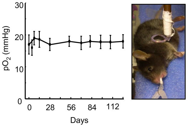
Long-term monitoring of in situ pO2 at the site of transplanted skeletal myoblasts (SM) in infarcted mouse hearts. Myocardial tissue pO2 from mice (N=5) implanted with LiNc-BuO in the mid-ventricular region without left anterior descending coronary artery ligation. Data show the feasibility of pO2 measurements for more than 3 months after implantation. Reprinted with permission from ref . Copyright 2008 Springer.
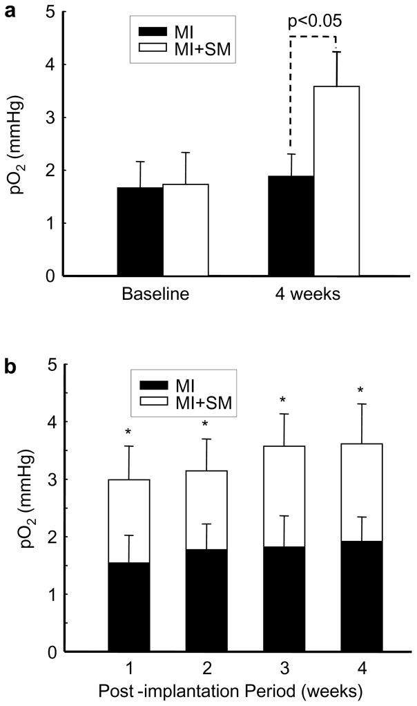
Myocardial pO2 in the infarcted heart at site of cell transplantation. Myocardial pO2 values were measured repeatedly for 4 weeks using in vivo EPR oximetry in mice hearts transplanted with LiNc-BuO-labeled skeletal myoblasts (SM) cells. a: Tissue pO2 at 4 weeks after treatment with SM cells (MI+SM) was significantly higher as compared to untreated (MI) hearts. b: The time-course values of myocardial pO2 measured from infarcted hearts (MI), and infarcted hearts treated with SM cells (MI+SM) are shown. Values are expressed as mean±SD (n=7 per group). *p<0.05 vs MI group. Reprinted with permission from ref . Copyright 2007 American Physiological Society.
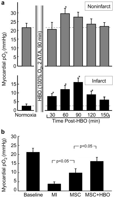
Hyperbaric oxygenation and myocardial pO2, in vivo. a: Myocardial pO2 in (noninfarcted and infarct) rat hearts measured before (normoxia) and after HBO. Data represent mean±SD obtained from 4 rats. The results show an increase in oxygenation levels reaching significance at 60 min followed by returning to baseline in about 2.5 hours in the noninfarcted hearts. In the infarcted hearts the oxygenation levels are significantly higher up to 2 hours post-treatment. It is interesting to note that a 5.8-fold increase in oxygenation is achieved in the infarct hearts after 90 min of HBO. b: Myocardial pO2 in rat hearts transplanted with stem cells at 2 weeks. The results (mean±SD; N=4 rats) show an increase in myocardial oxygenation in hearts treated with MSC and further enhancement in pO2 was observed in hearts treated with HBO. Reprinted with permission from ref . Copyright 2009 Elsevier.
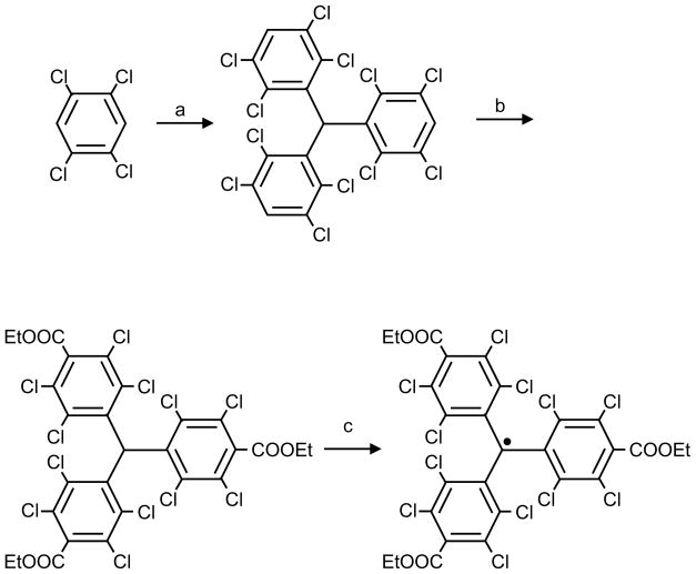
Synthesis of PTM-TE radical. Reagents and conditions: (a) CHCl3, AlCl3; (b) n-BuLi, TMEDA, ethyl chloroformate, 77%; (c) (1) NaOH, DMSO/Et2O, (2) I2, Et2O, 93%.
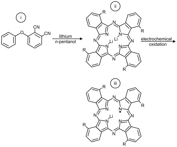
LiPc-α-OPh was synthesized by cyclotetramerization of 3-phenoxyphthalonitrile (i) in the presence of lithium pentoxide to obtain Li2Pc-α-OPh (ii) followed by electrochemical oxidation to form microcrystals of LiPc-α-OPh (iii).
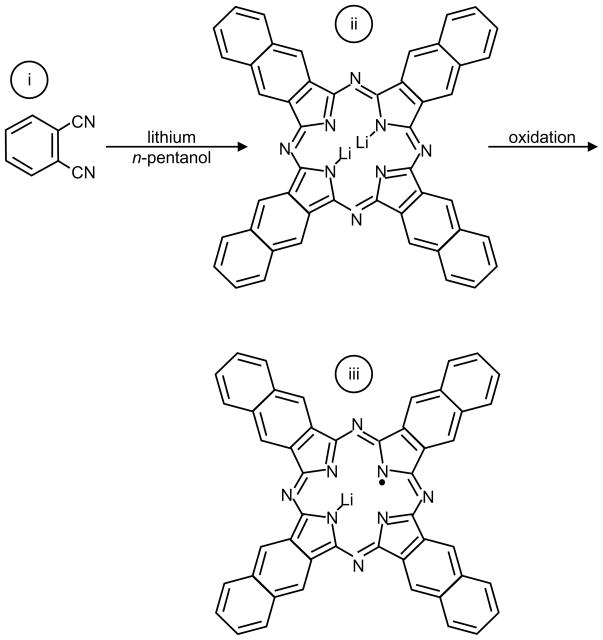
LiNc was synthesized by cyclotetramerization of 2,3-dicyano naphthalene (i), in the presence of lithium/pentanol to give Li2Nc (ii), followed by oxidation to form microcrystals of LiNc (iii).
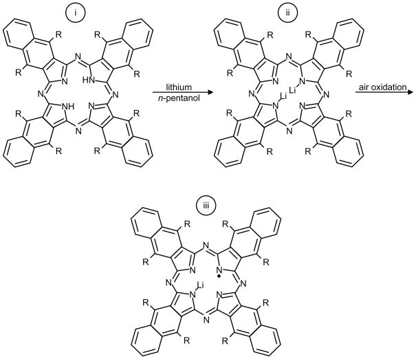
LiNc-BuO was synthesized from lithium metal and octa-n-butoxy-substituted naphthalocyanine (Nc-BuO) (i) in n-pentanol. Nc-BuO macrocyclic ligand reacted with lithium pentoxide (lithium metal in pentanol) to give dilithium octa-n-butoxy-naphthalocyanine (Li2Nc-BuO) (ii), followed by oxidation to give LiNc-BuO radical (iii) which formed as needle-shaped dark-green microcrystals.
References
-
- Lane N. Oxygen: The Molecule that Made the World. Oxford University Press; Oxford: 2002.
-
- Falkowski PG. Science. 2006;311:1724. - PubMed
-
- Jiang YY, Kong DX, Qin T, Zhang HY. Biochem Biophys Res Commun. 2009 - PubMed
-
- Raymond J, Segre D. Science. 2006;311:1764. - PubMed
-
- Kulkarni AC, Kuppusamy P, Parinandi N. Antioxid Redox Signal. 2007;9:1717. - PubMed
Publication types
MeSH terms
Substances
Grants and funding
LinkOut - more resources
Full Text Sources
Other Literature Sources
