. 2010 May;103(5):2783-93.
doi: 10.1152/jn.00730.2009. Epub 2010 Mar 10.

Brief sounds evoke prolonged responses in anesthetized ferret auditory cortex

Affiliations

Brief sounds evoke prolonged responses in anesthetized ferret auditory cortex

Robert A A Campbell et al. J Neurophysiol. 2010 May.

Abstract

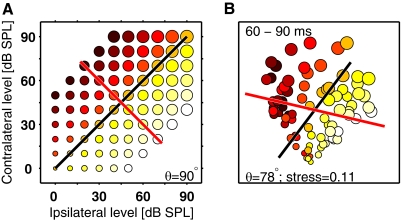
Neurons in the auditory cortex of anesthetized animals are generally considered to generate phasic responses to simple stimuli such as tones or noise bursts. In this paper, we show that under ketamine/medetomidine anesthesia, neurons in ferret auditory cortex usually exhibit complex sustained responses. We presented 100-ms broad-band noise bursts at a range of interaural level differences (ILDs) and average binaural levels (ABLs), and used extracellular electrodes to monitor evoked activity over 700 ms poststimulus onset. We estimated the degree of randomness (noise) in the response functions of individual neurons over poststimulus time; we found that neural activity was significantly modulated by sound for up to approximately 500 ms following stimulus offset. Pooling data from all neurons, we found that spiking activity carries significant information about stimulus identity over this same time period. However, information about ILD decayed much more quickly over time compared with information about ABL. In addition, ILD and ABL are coded independently by the neural population even though this is not the case at individual neurons. Though most neurons responded more strongly to ILDs corresponding to the opposite side of space, as a population, they were equally informative about both contra- and ipsilateral stimuli.


Figures

Fig. 1.
Fig. 1.
Sensitivity in interaural level difference (ILD) and average binaural level (ABL) in the ferret auditory cortex. A: the black points show the 80 sound level combinations used in this study. The gray lines are the axes along which ILD and ABL vary. B–E: responses of one unit in ferret auditory cortex to the binaural stimulus set. B: response function derived from the first peak in the pooled PSTH (13–43 ms). The unit fired most for intense contralateral sounds, as indicated by the white region in the response function. C: pooled PSTH representing the response summed across all 80 tested sound level combinations. The stimulus was presented during the first 100 ms (gray box). D: raster plot showing the pooled PSTH broken down by sound level combination. Each point represents a spike and each row of spikes represents a different stimulus presentation. In this case, each sound level combination (i.e., condition) was presented 10 times, and different conditions are segregated by the horizontal lines (during recordings the stimulus conditions were randomly interleaved not presented in blocks). The sound level combination is indicated by the numbers along the y axis, with “C” meaning contralateral sound level (dB SPL) and “I” meaning ipsilateral sound level. For clarity, only every other stimulus condition is labeled. The responses do not show evidence of adaptation and are fairly homogenous within conditions. This is highlighted by the inset plot (E), which shows 17 of the conditions in greater detail.
Fig. 2.
Fig. 2.
Three examples showing how binaural response properties change as a function of time. Each case shows the pooled PSTH of one unit with spike rate calculated over 5-ms bins. We extracted 13 binaural response functions along the PSTH using a series of 30-ms windows, which are highlighted as darker regions along each PSTH. The binaural response functions derived from these time slices are shown below each PSTH. The response functions are in the same format as Fig. 1B, but the gray scale of each function is normalized to the range of values for that time slice. The number above each response function indicates the window start time in milliseconds. The number below each response function is the z score indicating its smoothness, which is related to the signal-to-noise ratio of the response function (see main text for details). z scores less than −2.5 were taken to be significantly smoother than expected by chance and these are denoted in bold text. Significant time windows are highlighted on the PSTH in dark gray.
Fig. 3.
Fig. 3.
Distribution of smoothness scores over the neural population. A: the incidence of significant bins (black rectangles) for each unit. Units are arranged so that those with similar patterns of significant bins are adjacent to each other. The response of each unit is divided into 23 nonoverlapping time slices. Those time bins with z scores < −2.5 are filled black. B: the proportion of units exhibiting a nonrandom response function at each time bin (shaded region). Solid line, the cumulative proportion of all significant response windows over time. C: box plots of the observed smoothness z scores from all 310 units at each 30-ms time bin. For example, the box plot at t = 0 ms describes data in the 0- to 30-ms time window. Circles show the median; boxes, the interquartile range; and whiskers, 2.7 SD. Open circles, values >2.7 SD, which are jittered along the abscissa to aid visualization. Dotted lines indicate z = ±2.5, the significance cutoff used in previous figures. The observed z scores at each time point either have negative medians or are skewed toward negative values, which indicate smoother response profiles.
Fig. 4.
Fig. 4.
Classification of ILD and ABL over time using cross-validated multiple discriminant analysis (MDA). A: confusion matrices summarizing classification accuracy in ILD and ABL (see main text) for 5 example time windows. B: classification accuracy in bits derived from sequential 30-ms time windows. Accuracy is broken down into ILD (red) and ABL (black). C: classification accuracy expressed as the mean absolute error magnitude for ILD (red) and ABL (black). Shaded error bars show 1.96 SD of the bootstrapped chance distribution (see main text).
Fig. 5.
Fig. 5.
Population responses in multidimensional scaling (MDS) space. A: schematic of the stimulus space (Fig. 1A) where color represents ILD and circle diameter represents ABL. Under ideal conditions, one would expect 2-dimensional (2-D) MDS on the neural population responses (see main text) to produce a plot resembling this. The lines are generated by linear regression and indicate the directions that account for the most variance in ILD (red) and ABL (black). θ, the angle between the lines, is equal to 90° because ILD and ABL are orthogonal dimensions in stimulus space. B shows the results of an MDS projection from the 60- to 90-ms time window (part of the onset response) presented in the same format as A. The neural population data produce a map remarkably similar to the stimulus space. ILD and ABL vary in a systematic manner in neural space and the regression lines indicate that these variables are represented along largely orthogonal directions (θ = 78°). Information about these variables is therefore encoded largely independently. The MDS projection provides a good representation of the data because stress, a measure of the success of the transformation, equals 0.11 (0 is a perfect reconstructions; see methods).
Fig. 6.
Fig. 6.
Representation of ILD and ABL by the neural population as a function of poststimulus time. A: an MDS projection from the 150- to 180-ms time window. As in Fig. 5, ILD is represented by color and ABL by the size of the circles. The red line describes the direction in which ILD varies most and the black line the direction in which ABL varies most. The angle between these lines is 87°, indicating that the variables are represented independently. B and C: the distribution of the data around the ABL and ILD regressions, respectively. Each plot shows the predicted value of the parameter in MDS space as a function of the true value. An R2 of 1 would indicate that the neural population could perfectly predict the stimulus. At this time point accuracy is high. D–F: data for the 240- to 270-ms time window. G–I: data for 570- to 600-ms window. At the longer latencies post stimulus onset, there is still a substantial quantity of ABL information (H), whereas ILD information is no longer present (I). J: variation in R2 as a function of poststimulus time for ILD (red) and ABL (black). ILD information drops sharply at ∼240 ms, whereas ABL information drops off gradually over time and persists for much longer. Blue points shows the angle between the regression lines as a function of time. Time points with R2 <0.3 for ILD or ABL are shown as a dashed line.

Similar articles

Cited by

References

    1. Anderson J, Lampl I, Reichova I, Carandini M, Ferster D. Stimulus dependence of two-state fluctuations of membrane potential in cat visual cortex. Nat Neurosci 3: 617–621, 2000. - PubMed
    1. Arieli A, Sterkin A, Grinvald A, Aertsen A. Dynamics of ongoing activity: explanation of the large variability in evoked cortical responses. Science 273: 1868–1871, 1996. - PubMed
    1. Bajo VM, Nodal FR, Bizley JK, Moore DR, King AJ. The ferret auditory cortex: descending projections to the inferior colliculus. Cereb Cortex 17: 475–491, 2007. - PMC - PubMed
    1. Bartlett EL, Wang X. Long-lasting modulation by stimulus context in primate auditory cortex. J Neurophysiol 94: 83–104, 2005. - PubMed
    1. Bartho P, Curto C, Luczak A, Marguet SL, Harris KD. Population coding of tone stimuli in auditory cortex: dynamic rate vector analysis. Eur J Neurosci 30: 1767–1778, 2009. - PMC - PubMed

Publication types

LinkOut - more resources