Hippocampal replay is not a simple function of experience

Abstract

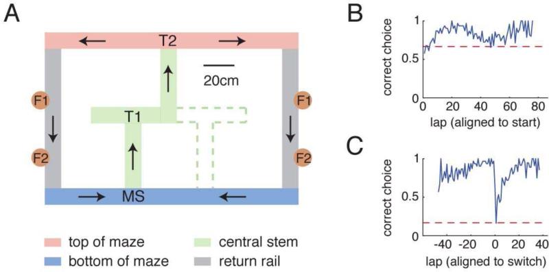
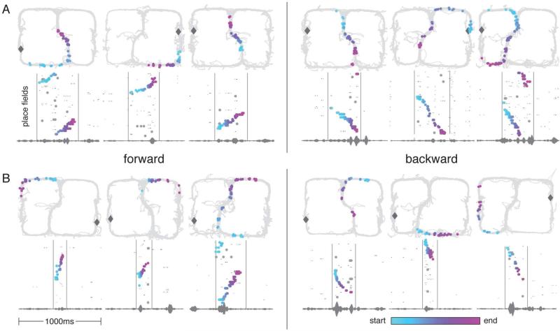
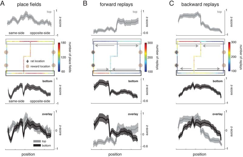
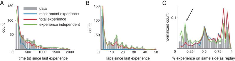
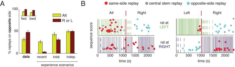
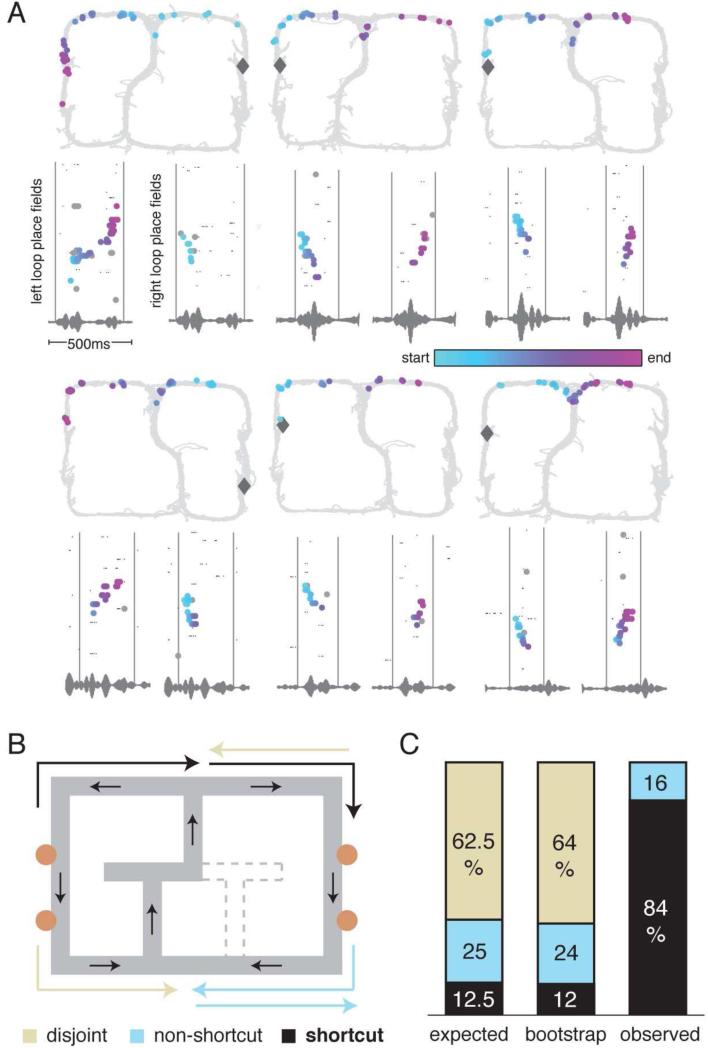
Replay of behavioral sequences in the hippocampus during sharp wave ripple complexes (SWRs) provides a potential mechanism for memory consolidation and the learning of knowledge structures. Current hypotheses imply that replay should straightforwardly reflect recent experience. However, we find these hypotheses to be incompatible with the content of replay on a task with two distinct behavioral sequences (A and B). We observed forward and backward replay of B even when rats had been performing A for >10 min. Furthermore, replay of nonlocal sequence B occurred more often when B was infrequently experienced. Neither forward nor backward sequences preferentially represented highly experienced trajectories within a session. Additionally, we observed the construction of never-experienced novel-path sequences. These observations challenge the idea that sequence activation during SWRs is a simple replay of recent experience. Instead, replay reflected all physically available trajectories within the environment, suggesting a potential role in active learning and maintenance of the cognitive map.

Figure 1

(A) The two-choice T maze. The maze had two possible physical configurations, the second indicated by dotted green lines. Noteworthy locations on the maze are labeled as follows: maze start (MS), turn 1 (T1), turn 2 (T2), feeder 1 (F1), and feeder 2 (F2). In addition the task entailed three reward contingencies reflecting a decision made at the second choice point (T2): animals were trained to turn left at the final choice, right at the final choice, or to alternate on a lap-by-lap basis. During recording days, the contingency was changed approximately midway through the task. Place fields did not change between contingencies (Figure S1). (B) Correctness of final choice (T2) aligned to the start of the session. If the task was alternation, the first lap was always deemed correct, so chance performance over all tasks is 2/3=66%. (C) Correctness of final choice (T2) aligned to the time of contingency switch. Chance of a pre-switch correct behavior being a correct behavior after the switch is 1/6=16%.

Figure 2

Examples of forward and backward replays. (A): Examples of same-side and central stem replays (3 fwd, 3 bwd). (B): Examples of opposite-side replays (3 fwd, 3 bwd). Gray diamond indicates the rat's location at the time of the replay. On the bottom panel of each subfigure, spikes are plotted by ordered place field (spatial firing field) center (along either a left or right loop of the maze) over a one second period (see Experimental Procedures). LFPs filtered between 180 Hz and 220 Hz are plotted at the bottom of the panel. Colored points indicate spikes that contribute positively to the sequence score of the replay according to the automatic sequence detection algorithm. The color of the spike indicates its relative time within the replay (light blue = early, light purple = late). Gray points are spikes that do not contribute positively to the score. For cells with multiple place fields, small black points are plotted at every place field center belonging to the cell (colored points occupy the place field center that contributes maximally to the score). Each colored point from the bottom panel is plotted on the 2D maze in the top panel at the location of its 2D place field center. Note that forward replays could begin near the rat's location ( A, left) or on the opposite side of the maze (B, left). Similarly, backward replays could begin near the rat's location (A, right) or on the opposite side of the maze (B, right). Backward replays occurred over parts of the environment that were rarely or never experienced in the reverse direction (Figures S2 and S3).

Figure 3

Spatial distribution of forward and backward replays. (A) Place field spatial distribution. (B) Forward replay spatial distribution. (C) Backward replay spatial distribution. Spatial distributions over the entire environment are shown in the second row. The first and third rows display the spatial distribution over the top and bottom of the maze (indicated by gray and black boxes in row 2), respectively. Spatial distributions over the top and bottom of the maze are overlaid for comparison in the fourth row. All mazes were flipped and aligned such that the animal's location was always on the left side of the maze (indicated by gray diamonds) at the time of the replay. Therefore, the spatial distribution on the left side of the maze reflect same-side replays and the distribution on the right reflect opposite-side replays. The pixel color indicates the total number of replays that represented that particular location in the environment. Errorbars in rows 1, 3, and 4 are SEMs over 31 sessions. Note that forward (fwd) and backward (bwd) replays preferentially represented certain portions of the maze, which could not be explained by the place field (pfs) distribution. Overall distributions were significantly different (p<10⁻⁷¹, fwd vs pfs; p<10⁻¹⁷⁶, bwd vs pfs; p<10⁻¹⁹⁷, fwd vs bwd; Kolmogorov-Smirnov tests).

Figure 4

Replay content is incompatible with scenarios based on recent experience or accumulated experience within a session. (A) Histogram showing the time elapsed since the last behavioral experience over each replayed trajectory. (B) Histogram showing the number of laps elapsed since the last behavioral experience over each replayed trajectory. (C) Histogram showing the proportion of total behavioral experience on the same side of the maze as each replayed trajectory at the time of the replay. The actual data (gray bars) is compared against three scenarios, where replay coverage is determined by recent experience (blue line), by accumulated experience (red line), or independent of experience (green line). The curves representing each scenario were constructed based on the animals’ actual behavior and replay times (see Experimental Procedures). Thus, the shapes of the curves reflect the finite session length and the behavioral contingencies. For example, the time-since-last-experience curve for the experience independent scenario (panel A) slopes downward due to the decreased probability that a replay event and the last experience over the replayed trajectory will be separated by 2000 s in a 2400 s recording session. Similarly in panel C, the experience independent curve has three peaks, reflecting the fact that experience was evenly distributed between left and right laps (during alternation) or was primarily on one side of the maze (during left or right-only contingencies). Note that in panel C, only the experience-independent scenario yields a good match to these data, because the other two scenarios fail to account for the peak in replays on the poorly-experienced side (black arrow). These results were replicated using a Bayesian decoding approach (Figure S4).

Figure 5

Influence of the behavioral contingency on the content of replay. (A) Proportion of opposite-side replays on alternation (A) vs right (R) or left-only (L) contingencies. The “Data” group is shown with all replays combined, as well as with forward (fwd) and backward (bwd) replays separately. Whereas the scenarios (described in text) all predicted a higher or equal proportion of opposite-side replays during alternation half-sessions, the data contained a significantly higher proportion of opposite-side replays during right or left-only half-sessions. [Errorbars are SEMs over half-sessions.] This result was replicated using a Bayesian decoding approach (Figure S4). (B) Examples of same-side and opposite-side replays on L and R contingencies versus an A contingency (2 sessions shown). For each session, the top panel shows left laps (vertical green lines) and replays (points) that occurred as the rat sat at the left reward locations. The bottom panel shows right laps (vertical purple lines) and replays (points) that occurred while the animal sat at the right reward locations. Dashed lines indicate error laps (e.g. the animal performs a right lap when only left laps are rewarded). Opposite-side replays are indicated by blue points, same-side replays by red points, and central stem replays by small gray points. Vertical red lines mark the contingency switch. X axis is time, Y axis is replay sequence score (see Experimental Procedures). Note the large number of blue points (opposite-side replays) during L or R contingencies compared to A. Thus, there was a bias for replaying non-local trajectories when they were infrequently experienced. This is in contrast to all three scenarios for replay content generation, including the experience-independent scenario.

Figure 6

Construction of novel shortcuts. (A) Examples of novel trajectories. On the bottom panels, spikes are plotted by ordered place field center for both left and right loops over the same 0.5 s period. The gray vertical lines mark the beginning and end of the shortcut sequence and capture the exact same period of time on both left and right loop raster plots (as can also be seen in the repeated LFP trace). The temporally color coded spikes (as described in the Figure 2 caption) are plotted on the 2D maze (top panels) to visualize the shortcut trajectories spanning the top of the maze. (B) Examples of a shortcut trajectory (black), a disjoint trajectory (beige), and a non-shortcut sequence (light blue). (C) Expected, bootstrapped, and observed distributions of disjoint, non-shortcut, and shortcut trajectories (see Experimental Procedures). This analysis shows that the observed shortcuts were extremely unlikely to arise from chance alignments of forward and backward replays, supporting the notion that rats can mentally construct spatially coherent, but never-experienced paths (see Figure S3 for paths experienced by each rat).

References

1. Ainge JA, Tamosiunaite M, Woergoetter F, Dudchenko PA. Hippocampal CA1 place cells encode intended destination on a maze with multiple choice points. J. Neurosci. 2007;27:9769–9779. - PMC - PubMed
1. Alvarez P, Squire LR. Memory consolidation and the medial temporal lobe: A simple network model. Proceedings of the National Academy of Sciences. USA. 1994;91:7041–7045. - PMC - PubMed
1. Alvernhe A, Van Cauter T, Save E, Poucet B. Different CA1 and CA3 Representations of Novel Routes in a Shortcut Situation. J. Neurosci. 2008;28:7324–7333. - PMC - PubMed
1. Buckner RL, Carroll DC. Self-projection and the brain. Trends in Cognitive Sciences. 2007;11:49–57. - PubMed
1. Buzsáki G. Two-stage model of memory trace formation: A role for “noisy” brain states. Neuroscience. 1989;31:551–570. - PubMed
Publication types