Linking structure and function in glaucoma

Abstract

The glaucomas are a group of relatively common optic neuropathies, in which the pathological loss of retinal ganglion cells causes a progressive loss of sight and associated alterations in the retinal nerve fiber layer and optic nerve head. The diagnosis and management of glaucoma are often dependent on methods of clinical testing that either, 1) identify and quantify patterns of functional visual abnormality, or 2) quantify structural abnormality in the retinal nerve fiber layer, both of which are caused by loss of retinal ganglion cells. Although it is evident that the abnormalities in structure and function should be correlated, propositions to link losses in structure and function in glaucoma have been formulated only recently. The present report describes an attempt to build a model of these linking propositions using data from investigations of the relationships between losses of visual sensitivity and thinning of retinal nerve fiber layer over progressive stages of glaucoma severity. A foundation for the model was laid through the pointwise relationships between visual sensitivities (behavioral perimetry in monkeys with experimental glaucoma) and histological analyses of retinal ganglion cell densities in corresponding retinal locations. The subsequent blocks of the model were constructed from clinical studies of aging in normal human subjects and of clinical glaucoma in patients to provide a direct comparison of the results from standard clinical perimetry and optical coherence tomography. The final formulation is a nonlinear structure-function model that was evaluated by the accuracy and precision of translating visual sensitivities in a region of the visual field to produce a predicted thickness of the retinal nerve fiber layer in the peripapillary sector that corresponded to the region of reduced visual sensitivity. The model was tested on two independent patient populations, with results that confirmed the predictive relationship between the retinal nerve fiber layer thickness and visual sensitivities from clinical perimetry. Thus, the proposed model for linking structure and function in glaucoma has provided information that is important in understanding the results of standard clinical testing and the neuronal losses caused by glaucoma, which may have clinical application for inter-test comparisons of the stage of disease.

Figure 1

A structure-function relationship between SAP visual sensitivity and histologically defined RGC density in monkeys with experimental glaucoma. (A) An example of the relationship for SAP visual sensitivity as a function of RGC density when both parameters are transformed to a logarithmic scale. Data for the control eyes are presented as open symbols and data for the lasered eyes are presented as filled symbols. The data for linear regression analysis on the data are presented in the inset (Adapted from Harwerth, et al., 2005). (B) The relationships between SAP visual sensitivity and RGC density for four retinal eccentricities, using the model described by equations 1 – 3. (C) The dynamic range of measurements by SAP based on the underlying RGC densities. The data for the normal RGC density as a function of eccentricity are based on the normal visual sensitivity at each eccentricity. The normal cell density decreased by 2 SD units represents the smallest loss of RGC density that would cause a statistically significant visual field defect. The cell density at zero sensitivity represents the RGC density at which SAP measurements fail and the RGC density cannot be assessed by clinical SAP. The distance between the lines for the cell densities minus 2 SD units and the cell densities at zero sensitivity represents the dynamic range of measurement.

Figure 2

A comparison of the relationships between the modeled and measured RGC densities. (A) Application of the NLM described by equations 1 – 3 and (B) application of the LM described by equations 4 and 5 for the translation between SAP visual sensitivity and RGC density that were used to obtain the predicted RGC densities. Symbols for data for each of the 4 eccentricities are indicated by the symbol legend. For each method of relating visual sensitivity to neuron density, the 1:1 relationship is illustrated by the solid line and the 95% limits of agreement are illustrated by the dashed lines. The upper inset histograms present the residual errors between modeled and measured data, with the mean residual deviation (MRD) and the standard deviation (SD) of the distribution shown on the graph. Other statistical goodness-of-fit indices that are inset to the graph represent the coefficient of determination (R²), the mean absolute deviation (MAD), and root mean squared deviation (RMSD)

Figure 3

SAP and contrast sensitivity perimetry for a monkey (OHT-46) with laser-induced experimental glaucoma. The gray-scale plot for SAP shows the peripheral locations for contrast sensitivity testing by the filled symbols. The contrast sensitivity functions at each location for OHT-46 are presented and, for comparison, the mean function for control eyes. The fitted functions are a two-parameter, low-pass model used to determine the height (peak contrast sensitivity) and location (cut-off spatial frequency) of the contrast sensitivity function. The total deviations from expected sensitivities for SAP of normal monkey eyes by behavioral testing with the Humphrey Field Analyzer (HFA) are inset on the graphs.

Figure 4

The peak contrast sensitivity as a function of the cut-off spatial for monkeys with visual field defects from experimental glaucoma for central and peripheral visual field locations (A–D), shown in the graph labels. Data from six monkeys are included, with repeated measures as their visual field defects progressed. To present the main effects more clearly, the data for peak contrast sensitivities have been combined into 8 bins of spatial frequency with the mean ±SD plotted for each bin. The two-line functions were fitted to demonstrate a shift in the locations of the functions without a reduction in height, i.e., loss of contrast sensitivity. For the two-line function, with one segment was determined by linear regression over the four lowest spatial frequencies (slopes shown on the plot), and the other segment with a zero slope was placed at the mean contrast sensitivity for the three highest spatial frequencies.

Figure 5

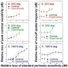
A comparison of visual defects measured by contrast sensitivity with Gabor patches versus SAP with Goldmann III stimuli for 3 peripheral visual field locations (A–F) shown in the graph labels. To compare the contrast sensitivity data to SAP data, the peak contrast sensitivities and cutoff frequencies were transformed to a dB scale by 10-times their logarithmic values. The losses of peak contrast sensitivity or cut-off spatial frequency represent the measured minus the expected values at each location, based on the data for normal eyes presented in Fig. 3. The relative loss of sensitivity by clinical perimetry represent the total deviations from expected sensitivities for SAP of normal monkey eyes by behavioral testing.

Figure 6

A plan for mapping SAP 24-2 visual field locations and RNFL thickness measures onto the ONH, in order to correlate structural and functional measures of glaucomatous neuropathy. The SAP 24-2 visual field locations were divided into 10 equal areas (A), with each representing 51 samples of the standard (512 point) OCT scan of the RNFL (B) or a 36 deg sector of the ONH (C). The curve of RNFL thickness plotted in panel B is referred to by the acronym “TSNIT” from the relationship between the pixel number (lower scale) in the OCT scan and the RNFL location of the scan (upper labels). The RNFL thickness measures start (pixel 1) at a retinal location that is Temporal to the ONH, the measurement progresses sequentially to the Superior, Nasal, Inferior, and back to the Temporal starting location (pixel 512) for a TSNIT representation of RNFL thickness. (D) Analogous TSNIT functions for the predicted numbers of somas and axons in the RNFL based on the structure-function model (see text, functions 1– 5). The functions represent the normative data from control eyes of monkeys to compare the number of RGC somas derived from the perimetry measurements (squares) and the number of RGC axons derived from OCT measurements of RNFL thickness (circles) for each of the 10 sectors of the optic nerve head (Adapted from Harwerth, et al., 2007).

Figure 7

An application of the structure-function model for relating SAP visual sensitivity and OCT fiber layer thickness for control and laser-treated eyes of monkeys that is described in the text (equations 1 – 5). The number of RGC axons derived from RNFL data as a function of the number of RGC somas from visual field data for corresponding sectors of SAP and OCT measurements. The correspondence between the subjective and objective measurements was evaluated by the 1:1 relationship that is illustrated by the solid line and the 95% limits of agreement that are illustrated by the dashed lines. The upper inset histogram presents the residual differences between the estimated populations of neurons, with the mean residual deviation (MRD) and the standard deviation (SD) of the distribution shown on the graph. The line superimposed on the histogram is a Gaussian distribution with parameters based on the MRD and SD of the distribution of residuals. The other statistical goodness-of-fit indices shown in the inset of the graph represent the coefficient of determination (R²), the mean absolute deviation (MAD), and root mean squared deviation (RMSD) of the axon versus soma data.

Figure 8

Adapting the structure-function models for experimental glaucoma to human subjects by including age-dependent and stage-dependent variables for objective measures of RGC axons. (A) The decrease in the numbers of RGC somas as a function of age, using the modified relationships for the human eye (equations 6 – 9) is illustrated by the steeper linear function (parameters shown in the inset) and the decrease in RGC axons based on a constant density of axons in the RNFL is illustrated by the more shallow linear function (parameters shown in the inset). (B) To obtain agreement between the populations of RGC somas and axons, a model for the age-related thinning of the RNFL was proposed, in which the total RNFL thickness at each age represents the sum of two components of the total thickness, i.e., an age-dependent loss of neuronal tissue and a compensating increase of non-neuronal tissue, with the resulting axonal density in the RNFL and numbers of axons over a RNFL sector derived from equations 10 and 11 (figure adapted from Harwerth and Wheat, 2008). (C) The loss of neurons as a function of the perimetric index of disease severity (MD) based on the SAP visual sensitivities (steeper function, with parameters shown in the inset) or the OCT data with only compensation for the patient’s age (shallower slope, with parameters shown in the inset). (D) To obtain agreement between the populations of RGC somas and axons, a model for stage-dependent changes in RNFL thickness was proposed. The model is illustrated by data for 65 year-old patients, in which the total RNFL thickness at each stage of disease is determined by the sum of two components of the thickness, i.e., neuronal tissue thickness that decreases with the stage of disease and non-neuronal tissue that is relatively constant. The derived stage-dependent correction is described by equations 12 and 13.

Figure 9

Applications of the structure-function model to relate neuronal populations as measured by OCT and SAP. Data are presented for normal controls (A) and glaucoma suspects and patients with glaucoma (B). The details for the analyses and statistical indices for the goodness-of-fit are as described for Fig. 7.

Figure 10

Structure versus function relationships in glaucoma analyzed by nonlinear and linear models for the patients from the University of Houston (UH_pats). (A) The NLM for relating the numbers of RGC axons and RGC somas that is described by equations 6 –13. The analysis was applied separately to SAP and OCT data representing the superior and inferior hemi-fields, with resulting statistical indices shown as graph insets. (B) The SLM for relating the RNFL thickness to the relative visual sensitivity from SAP measurements. The methods described by Hood and Kardon (2007) and reproduced by equations 14 – 17 were used to analyze data for the superior and inferior fields separately. The functions superimposed on the data were constructed using parameters from Hood and Kardon (2007).

Figure 11

Structure versus function relationships in glaucoma analyzed by nonlinear and linear models for the patients from the Bascom Palmer Eye Institute (BP_pats). All of the other details are as described for Fig. 10.

Figure 12

Applications of the NLM and SLM to predict RNFL thickness from SAP measures of visual sensitivity for the UH_pats. (A) To derive the relationship using the NLM, the total number of RGC somas for the superior and inferior fields, via equations 6 – 9, was substituted for the number of axons in equation 13 to back-solve for the mean thickness in equation 11. (B) The relationships for the SLM were derived from the thickness vs. sensitivity relations (equations 14 – 17) that are shown in Figs. 10 and 11 for the superior and inferior fields. The evaluations of the goodness-of-fit between the modeled and measured thicknesses for the NLM and SLM are the same as described for Fig. 7.

Figure 13

Applications of the NLM and SLM to predict RNFL thickness from SAP measures of visual sensitivity for the BP_pats. All of the other details are as described for Fig. 12.

Figure 14

An example of a method for mapping perimetric neural losses onto the TSNIT curve of RNFL thickness. The plan for mapping SAP areas onto sectors of the OCT scan described in Fig. 6, was used to derive an estimate of RNFL thickness from SAP measurements (A) and compared to the measured thickness from OCT measurements (B). The results for a glaucoma suspect with normal SAP and OCT are presented (C), with the RNFL scan shown by the thick solid line and the 95% CIs, based on three repeated measures, as the thin lines. The mean RNFL thicknesses from the OCT measurements are indicated by the solid circle at the mid-point of each sector and the RNFL thicknesses that were predicted from the corresponding SAP measurements are presented as the solid square symbols.

Figure 15

Examples of mapping perimetric neural losses onto the TSNIT curve of RNFL thickness for a patient with early glaucoma (A,B) and a patient with advanced glaucoma (C,D). The details of comparing the subjective and objective data are as described for Fig. 14.

Figure 16

The relationship between the RNFL thicknesses predicted from SAP measurements as a function of thicknesses measured by OCT. Data from the UH_pats (A) and BP_pats (B) were analyzed separately. The symbols are shaded to indicate the SAP and RNFL sectors represented, as illustrated in Fig. 6. The statistical indices to evaluate the goodness-of-fit between the modeled and measured thicknesses for the UH_pats and BP_pats are the same as described for Fig. 7.

References

1. Alamouti B, Funk J. Retinal thickness decreases with age: an OCT study. Br J Ophthalmol. 2003;87:899–901. - PMC - PubMed
1. Anderson AJ, Johnson CA, Fingeret M, et al. Characteristics of the normative database for the Humphrey matrix perimeter. Invest Ophthalmol Vis Sci. 2005;46:1540–1548. - PMC - PubMed
1. Anderson DR. Perimetry, With and Without Automation. 2. St. Louis: C.V. Mosby, Co; 1987.
1. Anderson DR, Knighton RW. Perimetry and acuity perimetry. In: Shields MB, Pollack IP, Kolker AE, editors. Perspectives in Glaucoma. Thorofare, NJ: Slack, Inc; 1988. pp. 59–70.
1. Ansari EA, Morgan JE, Snowden RJ. Psychophysical characteristics of early functional loss in glaucoma and ocular hypertension. Br J Ophthalmol. 2002;86:1131–1135. - PMC - PubMed
Publication types