Quantitative analysis of cryo-EM density map segmentation by watershed and scale-space filtering, and fitting of structures by alignment to regions

Abstract

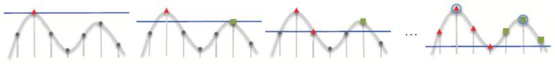
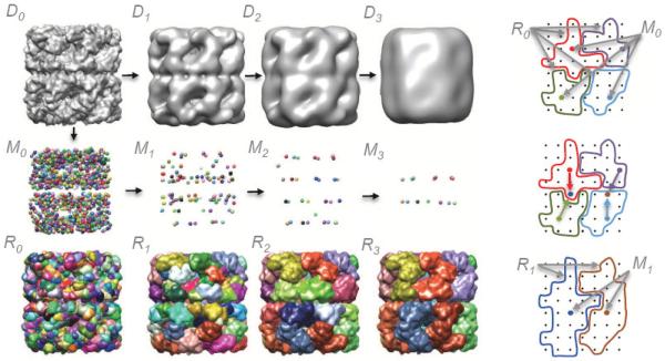
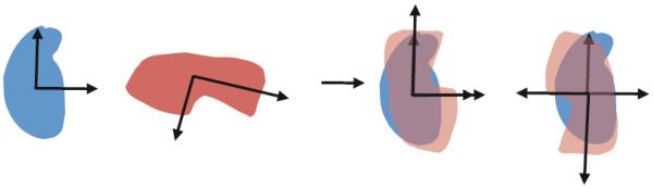
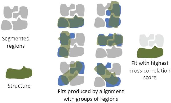
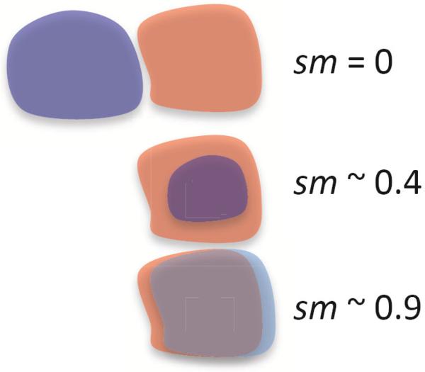
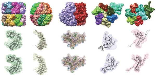
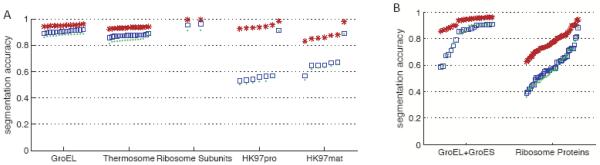
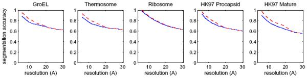
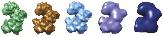
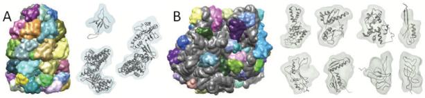
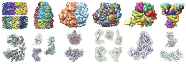
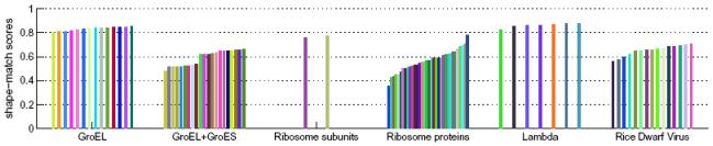
Cryo-electron microscopy produces 3D density maps of molecular machines, which consist of various molecular components such as proteins and RNA. Segmentation of individual components in such maps is a challenging task, and is mostly accomplished interactively. We present an approach based on the immersive watershed method and grouping of the resulting regions using progressively smoothed maps. The method requires only three parameters: the segmentation threshold, a smoothing step size, and the number of smoothing steps. We first apply the method to maps generated from molecular structures and use a quantitative metric to measure the segmentation accuracy. The method does not attain perfect accuracy, however it produces single or small groups of regions that roughly match individual proteins or subunits. We also present two methods for fitting of structures into density maps, based on aligning the structures with single regions or small groups of regions. The first method aligns centers and principal axes, whereas the second aligns centers and then rotates the structure to find the best fit. We describe both interactive and automated ways of using these two methods. Finally, we show segmentation and fitting results for several experimentally-obtained density maps.

Figure 1

From left to right, the images illustrate the first three and the last step during the immersive watershed algorithm for a 1D map. The smooth curve represents the underlying density function, which is discretized at evenly spaced grid points. Each point is drawn at a height proportional to its density value. The algorithm considers each point in order of decreasing density value: the point is added to a new region when none of its adjacent points are already in an existing region, or it is added to an existing region if it is adjacent to a point already in that region. In the end, two regions result in this example, containing either the points labeled with red triangles or the points labeled with green squares. Each region thus corresponds to a local density maximum (circled in the right-most image), which is the first point added to it. The points on the boundaries between the regions are points with the lowest density between local maxima.

Figure 2

The watershed segmentation of a density map, D₀, is a set of regions, R₀, with regions corresponding to points positioned at every local density maxima, M₀. Density maps are shown using iso-surfaces, regions are drawn using smooth surfaces that enclose contained voxels, and points of local density maxima are drawn using spheres. Grouping by scale-space filtering moves the points in M₀ by steepest ascent to local density maxima in D₁, yielding new points M₁. When two or more points in M₁ coincide, the corresponding regions are grouped, as shown in the images on the right, producing R₁. R₃ results after two more smoothing and grouping steps, in which each region corresponds to a single protein. The illustrated density map was generated from PDB:1xck at 10Å resolution.

Figure 3

Illustration of the principal axes transform for 2D shapes. The transform aligns centers of mass and principal axes. The signs of the principal axes are ambiguous; thus two alignments are possible in this 2D example.

Figure 4

A structure is aligned with automatically generated groups of segmented regions, producing many potential fits. The fit with the highest cross-correlation score is taken.

Figure 5

Illustration of the shape-match score, which is used to quantitatively measure the difference between two regions. The score is 0 when the regions are disjoint, and 1 only when they cover exactly the same area.

Figure 6

Segmented regions in 5 simulated density maps are shown on the top row; from left to right, they are GroEL, thermosome, Ribosome subunits, HK97 procapsid asymmetric unit (ASU), and HK97 mature capsid ASU. On the middle row, a single segmented region from each map is shown using a transparent surface, along with the structure of the corresponding protein or subunit shown as a ribbon. The bottom row shows regions resulting from grouping regions R₀ based on which protein-masked or subunit-masked region they overlap the most, and hence giving the maximum accuracy that could be attained by grouping watershed regions.

Figure 7

(A) Segmentation accuracies for the 5 simulated density maps shown in Figure 6. (B) Segmentation accuracies for simulated density maps of GroEL+GroES and Ribosome. Accuracies obtained with the grouping by scale-space filtering method are plotted with blue squares, accuracies obtained with the smoothing and sharpening method [31] are shown with green dots, and maximum accuracies attainable by grouping watershed regions are plotted with red asterisks. The same parameters were used for the two smoothing-based methods; the grouping method presented in this paper achieves slightly better segmentation accuracies.

Figure 8

Segmentation accuracies for 5 density maps simulated at various resolutions (6Å-30Å, every 2Å). The highest segmentation accuracy (blue lines) and highest maximum watershed segmentation accuracy (dashed red lines) amongst all components in each density map is plotted vs. resolution. The plots show that segmentation accuracies drop as the resolution increases, and that at low resolutions, the accuracies obtained by multi-scale grouping are the same as the maximum watershed accuracies.

Figure 9

Protein-masked region and segmented regions corresponding to a single protein in simulated maps of GroEL at different resolutions. The protein-masked is the first from the left. The remaining segmented regions are from maps with resolutions of (left to right) 6Å, 10Å, 20Å, and 30Å.

Figure 10

(A) Segmented regions from the simulated density map of GroEL+GroES (PDB:1aon) are shown. In the barrel-section (GroEL), groups of 2-3 regions correspond to single proteins, whereas in the lid section (GroES), single regions correspond to each protein. Three of the resulting regions (transparent surfaces) and corresponding proteins, chains A, H, and O (ribbons) are shown. (B) Segmented regions from the density map of the E-coli ribosome (PDB:2aw4,2avy) are shown, using random colors for regions corresponding each of the 45 correctly fitted proteins, and grey for all remaining regions. 8 of these fitted proteins (ribbons) and corresponding regions (transparent surfaces) are also shown. The top row shows 2avy chains B,C,D,J, and bottom row shows 2aw4 chains F,G,P,R).

Figure 11

Segmented experimental density maps, from left to right: GroEL, GroEL+GroES, ribosome large/small subunits, ribosome RNA/proteins, bacteriophage lambda, and rice dwarf virus. The top row shows regions after segmentation, grouping by scale-space filtering, and finally grouping based on fitted structures when fitted structures overlap more than one region. The bottom row shows single regions as transparent surfaces and corresponding fitted structures as ribbons. The structures are, from left to right, PDB:1xck chain A, PDB:1aon chains A, H, and O, PDB:2avy and PDB:2aw4 all chains, PDB:2avy chains M,I,J (top) and PDB:2aw4 chains G,P (bottom), PDB:3bqw, and PDB:1uf2 chains A and C.

Figure 12

Shape-match scores between segmented regions for 5 cryo-EM density maps and protein/subunit masked regions. The cryo-EM map of the ribosome was segmented twice, first into larger and small subunits, and then into proteins and RNA.

References

1. Ludtke SJ, Baker ML, Chen D, Song J, Chuang DT, Chiu W. De novo backbone trace of GroEL from single particle electron cryomicroscopy. Structure. 2008;16:441–448. - PubMed
1. Ranson NA, Clare DK, Farr GW, Houldershaw D, Horwich AL, Saibil HR. Allosteric signaling of ATP hydrolysis in GroEL-GroES complexes. Nat Struct Mol Biol. 2006;13:147–152. - PMC - PubMed
1. Valle M, Zavialov A, Li W, Stagg SM, Sengupta J, Nielsen RC, et al. Incorporation of aminoacyl-tRNA into the ribosome as seen by cryo-electron microscopy. Nat Struct Mol Biol. 2003;10:899–906. - PubMed
1. Lander GC, Evilevitch A, Jeembaeva M, Potter CS, Carragher B, Johnson JE. Bacteriophage lambda stabilization by auxiliary protein gpD: timing, location, and mechanism of attachment determined by cryo-EM. Structure. 2008;16:1399–1406. - PMC - PubMed
1. Zhou ZH, Baker ML, Jiang W, Dougherty M, Jakana J, Dong G, et al. Electron cryomicroscopy and bioinformatics suggest protein fold models for rice dwarf virus. Nat Struct Mol Biol. 2001;8:868–873. - PubMed
Publication types
MeSH terms
LinkOut - more resources