Discrimination of communication vocalizations by single neurons and groups of neurons in the auditory midbrain

Abstract

Many social animals including songbirds use communication vocalizations for individual recognition. The perception of vocalizations depends on the encoding of complex sounds by neurons in the ascending auditory system, each of which is tuned to a particular subset of acoustic features. Here, we examined how well the responses of single auditory neurons could be used to discriminate among bird songs and we compared discriminability to spectrotemporal tuning. We then used biologically realistic models of pooled neural responses to test whether the responses of groups of neurons discriminated among songs better than the responses of single neurons and whether discrimination by groups of neurons was related to spectrotemporal tuning and trial-to-trial response variability. The responses of single auditory midbrain neurons could be used to discriminate among vocalizations with a wide range of abilities, ranging from chance to 100%. The ability to discriminate among songs using single neuron responses was not correlated with spectrotemporal tuning. Pooling the responses of pairs of neurons generally led to better discrimination than the average of the two inputs and the most discriminating input. Pooling the responses of three to five single neurons continued to improve neural discrimination. The increase in discriminability was largest for groups of neurons with similar spectrotemporal tuning. Further, we found that groups of neurons with correlated spike trains achieved the largest gains in discriminability. We simulated neurons with varying levels of temporal precision and measured the discriminability of responses from single simulated neurons and groups of simulated neurons. Simulated neurons with biologically observed levels of temporal precision benefited more from pooling correlated inputs than did neurons with highly precise or imprecise spike trains. These findings suggest that pooling correlated neural responses with the levels of precision observed in the auditory midbrain increases neural discrimination of complex vocalizations.

Fig. 1.

Single neurons in zebra finch mesencephalicus lateralis dorsalis (MLd) showed a range of responses to song. A: diagram of the zebra finch ascending auditory system and electrode placement. B: the waveform (top) and spectrogram (middle) of a single zebra finch song. Below the spectrogram, raster plots show spike trains collected from 8 neurons in response to multiple presentations of the song. Each line shows a single spike train and each tick represents the timing of a single action potential (AP). Each group of 10 spike trains shows the responses of a single neuron to 10 presentations of the song. For the song spectrogram, red represents high intensity and blue represents low intensity.

Fig. 2.

MLd neural responses discriminated among songs with a wide range of abilities. A: spike trains from a single neuron in response to 10 repetitions of 20 unique zebra finch songs. Each group of 10 lines shows the responses to 10 presentations of a single song. The songs were pseudorandomly interleaved during the experiment and the responses were organized here for visualization. For analysis, the spike trains were truncated to the duration of the shortest song (1.62 s; nonshaded region). B: spike trains from a second neuron in response to the same stimuli as in A. C: in the K-means and van Rossum metrics, spike trains were represented as points in a 1,620-dimensional space (one dimension for each millisecond of activity). For illustration, here the spikes in response to the first 3 songs were projected onto 2 dimensions (the first 2 principal components). Spike trains from song 1 are shown in green, song 2 in blue, and song 3 in red. The K-means algorithm was used to classify the spike trains into clusters based on spike train dissimilarity. The shape of the marker corresponds to cluster membership. For Neuron 1, spike trains evoked by each song belong to their own cluster, indicating high discriminability. D: for Neuron 2, cluster 3 contains spike trains from songs 1, 2, and 3, indicating that the spike trains produced by this neuron cannot perfectly discriminate among the 3 songs. Color and shape labels are the same as in C.

Fig. 3.

Four neurometrics were used to measure neural discriminability. A: within each metric, each dot represents the discriminability of a single neuron. Neurons were ordered independently for each neurometric, from lowest to highest performance. Error bars show the SD across 100 repetitions of each neurometric. The right panel shows the mean discrimination performance using each neurometric. Error bars are ±1SD. B: discriminability measured with the K-means and van Rossum metrics showed a strong correspondence (r = 0.95). C: discrimination using the K-means and Victor–Purpura metrics were also highly correlated at the single neuron level (r = 0.96). In B and C, solid lines are unity. D: discriminability measured with the K-means metric was correlated with response strengths (driven firing rate minus baseline firing rate) between 0 and 13 spikes/s (r = 0.69, P < 0.0001). E: K-means discriminability increased with spike train duration. Each gray line shows the discriminability of a single neuron; the black line shows the average for the population. F: discriminability decreased as the number of songs to discriminate increased. The solid black line shows the average discriminability for the population and the dashed line shows chance performance at each set size. G: as the number of songs to discriminate increased, the spike train duration necessary to maintain discriminability increased sublinearly. Performance is represented as color, ranging from 0 to 100% correct. The abscissa shows the number of songs to discriminate and the ordinate shows the spike train duration used in the K-means neurometric. The solid line represents the isodiscriminabiltiy contour of 56% correct, which was the average discriminability. The dashed line shows the linear prediction of spike train duration necessary to maintain this level of discriminabitliy, based on set sizes of 2–4 songs. The dotted-dashed line shows the linear prediction based on set sizes of 5–7 songs.

Fig. 4.

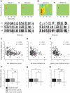
Neural discriminability was not correlated with spectral or temporal tuning. A: spectrotemporal receptive fields (STRFs) were calculated from neural responses to zebra finch song and estimates of the spectral and temporal tuning properties were computed from the STRF. The left panel shows the spectral projection of the STRF, from which we measured the best frequency (BF). Excitatory bandwidth (BW) was measured at the time of maximum excitation. The bottom panel shows the STRF's temporal projection, from which we measured the temporal modulation period (delay between the peaks of excitation and inhibition) and Excitatory–Inhibitory (EI) index, which was the normalized balance between excitation (shown in red) and inhibition (shown in blue). Positive values indicate stronger excitation than inhibition; negative values indicate stronger inhibition (range: −1 to 1). B: an example in which the STRF predicts the neural response to a novel sound (cc = 0.8; gray trace is the poststimulus time histogram (PSTH) of actual response; red trace is predicted response). C and D: discriminability is not correlated with best frequency (r = 0.11) or spectral bandwidth (r = 0.03). The top histograms in each panel show the distribution of BFs and BWs. E and F: discriminability is not correlated with the temporal modulation period (r = 0.01) or the EI index (r = −0.01). The right histogram shows the distribution of K-means discriminability, and corresponds to C–F. Dashed lines show the linear regression and the pink diamond represents the neuron from A.

Fig. 5.

Readout neurons that received input from 2 to 5 MLd neurons were simulated. A: a diagram of a readout neuron with 2 inputs (Neuron 1 and Neuron 2). B: the readout response was modeled using 3 different models. Example responses from each model are shown for the input spike trains labeled Neuron 1 and Neuron 2. C: average discriminability across the population of readout neurons as a function of the number of input neurons. D: discriminability of OR readout neurons with 2 inputs compared with the average discriminability of the 2 inputs. Solid line is the unity line. E: discriminability of OR readout neurons with 2 inputs compared with the input neuron that discriminated best. F: histogram showing the number of OR readout neurons that achieved gains in discriminability relative to the input neuron that discriminated best (P = 1.21 × 10⁻⁴, Wilcoxon signed-rank test).

Fig. 6.

Pairs of neurons with similar tuning properties obtained the largest gains in discriminability. A: 2 neurons with highly similar STRFs. Below the STRFs are 5 spike trains evoked by a single song for each of the neurons, as well as the output of the OR readout neuron. The rasters are highly similar for the two input neurons, which is reflected in the readout neuron. The gray bar shows qualitatively the increased signal strength obtained by the readout neuron. B: pair of neurons with dissimilar STRFs. Neuron 2 is the same as in A, but Neuron 1 has different tuning. For this pair, misaligned spike trains do not reinforce one another (gray bar). C: the gain in discriminability is correlated with the similarity of frequency tuning. The pairs in A and B are shown as a blue square and purple diamond, respectively. D: similar temporal tuning is correlated with gains in discriminability. E: pairs of neurons that produce similar spike train patterns have larger gains in discriminability than pairs of neurons with dissimilar spike train patterns. For C–E, the dashed lines show the linear regression. F–H: for the 3 parameters plotted in C–E, the gain in discriminability for the quartile of neurons with the most similar tuning (gray) and least similar tuning (white). Black bars show the gain in discriminability for readout neurons that receive input from identically tuned neurons. Error bars are ±1SD (*P ≤ 0. 01, Kruskal–Wallis test; **P ≤ 0.0002, Kruskal–Wallis test).

Fig. 7.

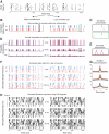
Simulating pairs of neurons with varying degrees of temporal precision and spike train similarity. A: a spike train from a real MLd neuron was used as a template from which simulated spike trains were generated. Each row shows the spiking response to one presentation of a single song; the bottom row (colored blue) was used as the template for the first simulated neuron in each pair (N1). B, D, F, and H: the left column in each panel shows a pair of neurons with highly correlated responses and the right column shows a pair of neurons with less correlated responses. B: temporal jitter was added to each “spike” in the N1 template to create a template for the second simulated neuron (N2). C: close-up of the amount of jitter introduced to the template in the left and right panels of B. D: the templates for N1 and N2 were smoothed with Hanning windows that ranged in width from 1 to 100 ms, resulting in continuous probability distributions. The blue distributions correspond to N1 and the red distributions to N2. The top, bottom, and middle panels show smoothing widths of 2, 8, and 20 ms. E: close-up of the amount of smoothing applied to the templates for N1 and N2. F: 10 spike trains were generated from each of the probability distributions. The top, middle, and bottom panels show spike trains for N1 and N2, generated from the respective distributions in D. G: the average shuffled autocorrelogram (SAC) of real MLd neurons (mean shown in black) compared with the SACs of simulated neurons (±1SD shown in red) with 2, 8, and 20 ms smoothing windows (from top to bottom). H: responses from an OR readout neurons that received simulated spike trains from N1 and N2 as inputs. From top to bottom, the readout neurons received input with progressively coarser temporal precision. Each panel shows 10 simulated responses to each of 5 songs.

Fig. 8.

Gain in discriminability for pairs of simulated neurons depended on spike train precision and response similarity. A: at each level of simulated precision, we measured the temporal precision as the peak of the SAC (coincidence index [CI]) normalized by the SAC half-width at half-height (W) (error bars are median with upper and lower quartiles). The diamond and dashed lines show the precision of real MLd neurons. Simulated neurons were grouped according to their observed temporal precision relative to real MLd neurons. B: within each group, the gain in discriminability was normalized to the gain achieved with highly similar inputs. The normalized gain was plotted against the similarity of the inputs.

References

1. Allen C, Stevens CF. An evaluation of causes for unreliability of synaptic transmission. Proc Natl Acad Sci USA 91: 10380–10383, 1994 - PMC - PubMed
1. Andoni S, Li N, Pollak GD. Spectrotemporal receptive fields in the inferior colliculus revealing selectivity for spectral motion in conspecific vocalizations. J Neurosci 27: 4882–4893, 2007 - PMC - PubMed
1. Arabzadeh E, Panzeri S, Diamond ME. Whisker vibration information carried by rat barrel cortex neurons. J Neurosci 24: 6011–6020, 2004 - PMC - PubMed
1. Aronov D, Reich DS, Mechler F, Victor JD. Neural coding of spatial phase in V1 of the macaque monkey. J Neurophysiol 89: 3304–3327, 2003 - PubMed
1. Barlow HB. Single units and sensation: a neuron doctrine for perceptual psychology? Perception 1: 371–394, 1972 - PubMed
Publication types
LinkOut - more resources