Optimized localization analysis for single-molecule tracking and super-resolution microscopy

Abstract

We optimally localized isolated fluorescent beads and molecules imaged as diffraction-limited spots, determined the orientation of molecules and present reliable formulas for the precision of various localization methods. Both theory and experimental data showed that unweighted least-squares fitting of a Gaussian squanders one-third of the available information, a popular formula for its precision exaggerates beyond Fisher's information limit, and weighted least-squares may do worse, whereas maximum-likelihood fitting is practically optimal.

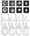
Figure 1

Point spread functions for four fixed fluorophores with different spatial orientations. (a–d): Fixed rhodamine molecules were imaged as described in Methods. (e–h): MLEwT applied to fixed probes (a–d) with 578 nm peak emission wavelength. We found orientations in polar angles, of 0.28, 0.60, 0.89, and 1.18 radians, respectively, for (e–h), and in azimuthal angles of 0.68, 2.23, 3.61, and 5.03. (i–l): Measured signal values compared to expected values. We binned the expected signals, and associated pixels with a bin if the expected signal falls within it. For each bin, the mean experimental signal is plotted against the expected signal. Error bars indicate the theoretical s.e.m. with which data should scatter about the straight line through the origin with unit slope. (m–p): Histograms of pixel fluctuations around their expected values. For each pixel in the experimental images (a–d), the fluctuation is the measured signal value minus its expected value, scaled by its theoretical r.m.s. deviation. For sufficiently large expected pixel signals, theory predicts the standard normal distribution (solid line) for the fluctuations. (q–t): Comparing the theoretical PSF to its analytical approximation (Supplementary Data). At (0,0) the two functions coincide. For each fit in (e–h), we show the percentile deviation of the analytical approximation from the theoretical PSF as a contour plot. Contour lines are plotted for 0.01, 0.1 (both solid lines), and −0.1 (dashed lines).

Figure 2

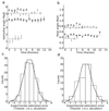
Demonstration of MLEwT on fixed fluorophores. (a): Time-series of repeatedly estimated azimuthal angles of four fixed fluorophores using MLEwT. Error bars indicate the theoretical r.m.s. deviation of each estimate, as caused by shot-noise only. For each time-series, the full lines represent the weighted mean value of the angle. (b): Polar angles for the same probes, obtained as in (a). (c): Histogram of fluctuations about the mean values of azimuthal and polar angles in seven time-series consisting of 68 estimates analyzed using MLEwT. Each fluctuation was re-scaled using the theoretical covariance matrix for it. Consequently, theory dictates a normal distribution with variance one, shown with the solid line. (d): Histogram of fluctuations about the mean values in time-series of distance estimates with MLEwT. For each of the seven probes used in (c), time series of Euclidean distances between the probe and all other probes fluorescing simultaneously were calculated. Fluctuations are given in units of their theoretical r.m.s. deviation, found by assuming shot-noise is the only source of statistical fluctuations. If this assumption is correct, theory dictates the normal distribution with unit variance, shown here as a solid line. (Because each probe contributes to several distance estimates, the latter are not fully independent statistically, but this "oversampling" of data merely reduces statistical noise in the shown histogram.)

Figure 3

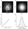
The point spread function of a 40-nm fluorescent bead. (a): 40 nm fluorescent beads were imaged as described in Methods. (b): Theoretical image: Obtained by applying MLEwT to the experimental image (a). We assumed circular polarization of the incident light. (c): Measured signal values compared to expected values. We binned the expected signals, and associated pixels with a bin having expected pixel values within it. For each bin, the mean experimental signal is plotted against the expected signal. The error bars indicate the theoretically predicted s.e.m. with which an experimental mean value is allowed to scatter about the straight line drawn through the origin with unit slope. (d): Histogram of pixel fluctuations around their expected values. For each pixel in the experimental image (a), the fluctuation is the measured signal value minus its expected value, scaled by its theoretical r.m.s. deviation. For a sufficiently large expected pixel signal, the actual signal value is approximately normally distributed. For such fluctuations, the theory dictates the normal distribution with variance one, shown with the solid line.

Figure 4

Comparing four estimators. (a–d): Time series of repeatedly measured distance between two fluorescent beads melted onto a cover slip. Notice the larger scatter in (d) compared to (c) and (c) compared to (a) and (b). (a): Distances obtained with MLEwT. (b): Distances obtained with MLEwG applied to the very same data. (c): Distances obtained with GME. (d): Distances obtained with WLS. (e): Power spectra of the four time series. The excess power at lowest frequencies may be due to Brownian motion of the beads. The plateau value at larger frequencies equals twice the variance of the point-source localization scheme. Curves: Fits of a Lorentzian plus a constant to experimental power spectra. Arrows: Plateau values according to theory (Supplementary Note). Note that the white arrow (MLEwT and MLEwG, undistinguishable) marks the information limit: All unbiased estimators have variances larger than or equal to this limit. Note also that Eq.(17) in Ref. violates the information limit when applied to the experimental data discussed here, hence must be wrong. (f): Histogram of fluctuations about the mean value in time-series of distance estimates with MLEwT. Each fluctuation was divided by the theoretical r.m.s. deviation for it. Consequently, theory dictates a normal distribution with variance one, shown with the solid line. (g): Same for MLEwG. (h): Same for GME. (i): Same for WLS, rescaled using Eq.(5). The width of the histogram compared to theory is due to low experimental values in some pixels.

References

1. Born M, Wolf E. Principles of Optics. New York: Cambridge University Press; 1999.
1. Barak LS, Webb WW. J. Cell Biol. 1982;95:846–852. - PMC - PubMed
1. Yildiz A, et al. Science. 2003;300:2061–2065. - PubMed
1. Okten Z, Churchman LS, Rock RS, Spudich JA. Nat. Struct. Mol. Biol. 2004;11:884–887. - PubMed
1. Betzig E, et al. Science. 2006;313:1642–1645. - PubMed
Publication types