. 2010 Jun;29(6):1310-20.
doi: 10.1109/TMI.2010.2046908. Epub 2010 Apr 8.

N4ITK: improved N3 bias correction

Affiliations

N4ITK: improved N3 bias correction

Nicholas J Tustison et al. IEEE Trans Med Imaging. 2010 Jun.

Abstract

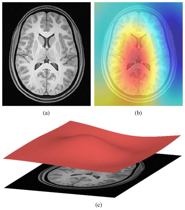
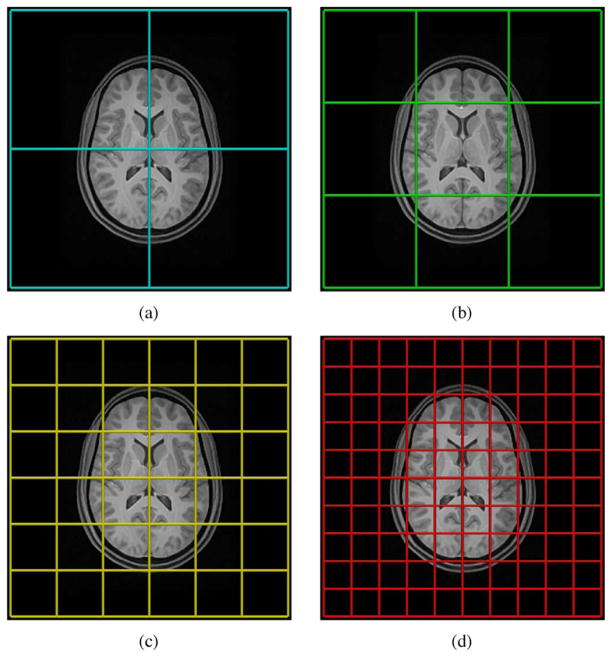
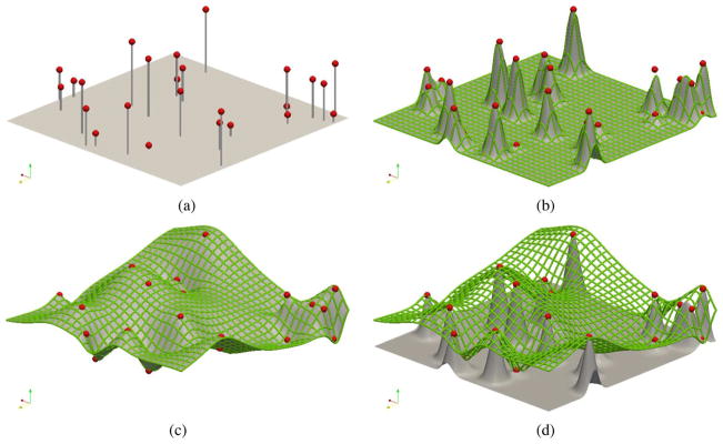
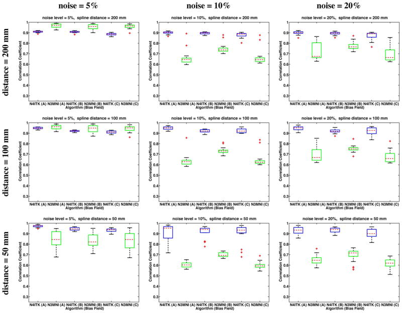
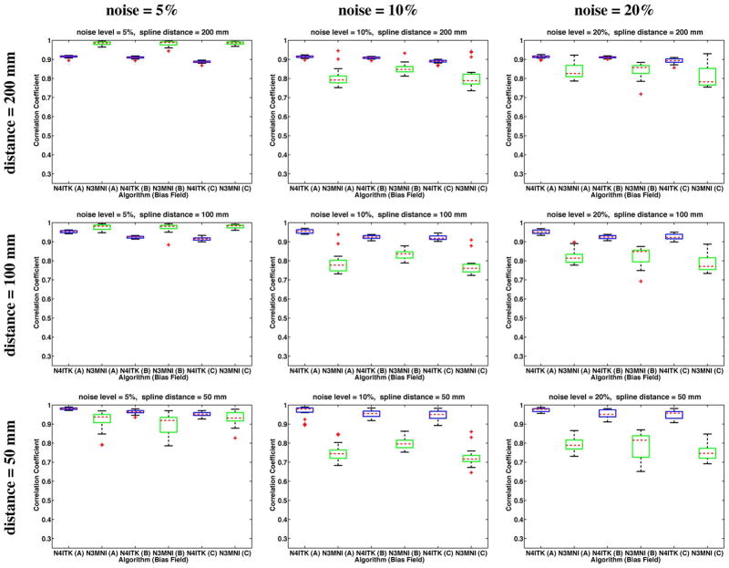
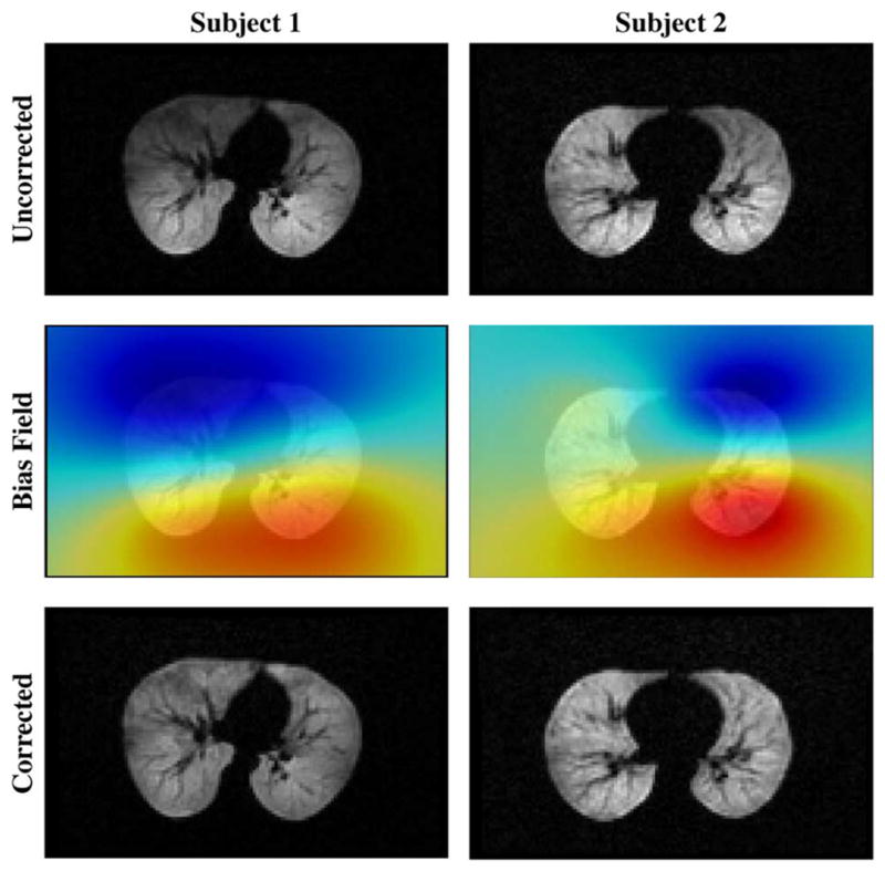
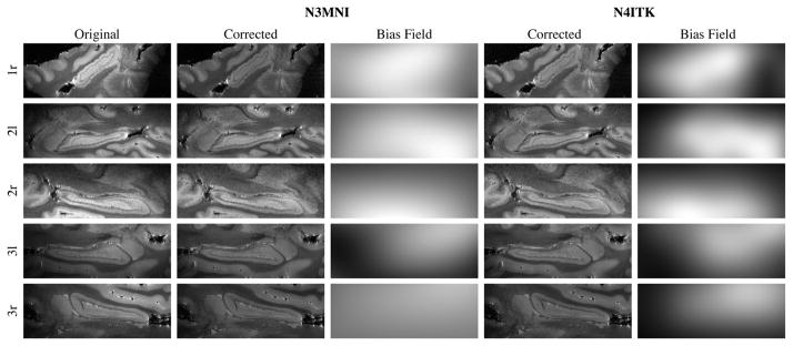
A variant of the popular nonparametric nonuniform intensity normalization (N3) algorithm is proposed for bias field correction. Given the superb performance of N3 and its public availability, it has been the subject of several evaluation studies. These studies have demonstrated the importance of certain parameters associated with the B-spline least-squares fitting. We propose the substitution of a recently developed fast and robust B-spline approximation routine and a modified hierarchical optimization scheme for improved bias field correction over the original N3 algorithm. Similar to the N3 algorithm, we also make the source code, testing, and technical documentation of our contribution, which we denote as "N4ITK," available to the public through the Insight Toolkit of the National Institutes of Health. Performance assessment is demonstrated using simulated data from the publicly available Brainweb database, hyperpolarized (3)He lung image data, and 9.4T postmortem hippocampus data.


Figures

Fig. 1
Fig. 1
(a) T1-weighted MR image exhibiting bias. (b) Several algorithms have been proposed to estimate the bias field which can then be used to “correct” the image. (c). Viewed as a surface, the low frequency modulation of the bias field is readily apparent.
Fig. 2
Fig. 2
Illustration of the spline distance parameter of N3 relative to typical brain anatomy. For uniform B-splines (which are employed by N3), spline distance, i.e., control point spacing, is identical with the mesh element size. Several commonly used N3 spline distances are overlaid on an axial brain slice: (a) 150 mm, (b) 100 mm, (c) 50 mm, and (d) 30 mm. Not shown is the default N3 control point spacing of 200 mm.
Fig. 3
Fig. 3
Comparison of fitting strategies for a simple 2-D scattered point set example. (a) Set of 25 scattered data points. (b) Highly localized approximation using a single level 32 × 32 element B-spline mesh. (c) Approximation by a hierarchy of B-spline mesh resolutions starting from a single B-spline mesh element and ending with a 32×32 element B-spline mesh. (d) Superposition of the fitted B-spline mesh from (c) and the fitted surface from (b) to illustrate the discrepancy in solutions.
Fig. 4
Fig. 4
20% bias field results: Correlation coefficient analysis for the BrainWeb data with varying levels of additive Gaussian noise and spline distances where the simulated bias fields were linearly rescaled to [0.9,1.1]. Results are paired by bias field with the results of N4ITK given in blue and the corresponding N3MNI results given in green. Although N3MNI performs comparatively well for the 5% noise level and spline distance = 200 mm, with increasing noise and increasing mesh resolution (i.e., decreased spline distance), N4ITK consistently achieves improved results.
Fig. 5
Fig. 5
40% bias field results: Correlation coefficient analysis for the BrainWeb data with varying levels of additive Gaussian noise and spline distances where the simulated bias fields were linearly rescaled to [0.8,1.2]. Results are paired by bias field with the results of N4ITK given in blue and the corresponding N3MNI results given in green. Although N3MNI performs comparatively well for the 5% noise level and spline distance = 200 mm, with increasing noise and increasing mesh resolution (i.e., decreased spline distance), N4ITK consistently achieves improved results.
Fig. 6
Fig. 6
Top row: Axial 3 Hp lung MRI from two subjects evidencing bias field artifacts. Middle row: The calculated bias field. Bottom row: Corrected images.
Fig. 7
Fig. 7
The first column gives 2-D sagittal views of postmortem hippocampi in three subjects (“r” denotes right hippocampus, “l” denotes left hippocampus). The second and third columns give the corrected image using N3MNI and the corresponding bias field whereas the results using N4ITK are provided in columns 4 and 5.

Similar articles

Cited by

References

    1. Belaroussi B, Milles J, Carme S, Zhu YM, Benoit-Cattin H. Intensity nonuniformity correction in MRI: Existing methods and their validation. Med Image Anal. 2006 Apr;10(2):234–246. - PubMed
    1. Hou Z. A review on MR image intensity inhomogeneity correction. Int J Biomed Imag. 2006;2006:1–11. - PMC - PubMed
    1. Vovk U, Pernus F, Likar B. A review of methods for correction of intensity inhomogeneity in MRI. IEEE Trans Med Imag. 2007 Mar;26(3):405–421. - PubMed
    1. Sled JG, Zijdenbos AP, Evans AC. A nonparametric method for automatic correction of intensity nonuniformity in MRI data. IEEE Trans Med Imag. 1998 Feb;17(1):87–97. - PubMed
    1. Arnold JB, Liow JS, Schaper KA, Stern JJ, Sled JG, Shattuck DW, Worth AJ, Cohen MS, Leahy RM, Mazziotta JC, Rottenberg A. Qualitative and quantitative evaluation of six algorithms for correcting intensity nonuniformity effects. Neuroimage. 2001 May;13(5):931–943. - PubMed

Publication types