

Quantitative modeling of Escherichia coli chemotactic motion in environments varying in space and time
- PMID: 20386737
- PMCID: PMC2851563
- DOI: 10.1371/journal.pcbi.1000735
Quantitative modeling of Escherichia coli chemotactic motion in environments varying in space and time
Abstract
Escherichia coli chemotactic motion in spatiotemporally varying environments is studied by using a computational model based on a coarse-grained description of the intracellular signaling pathway dynamics. We find that the cell's chemotaxis drift velocity v(d) is a constant in an exponential attractant concentration gradient [L] proportional, variantexp(Gx). v(d) depends linearly on the exponential gradient G before it saturates when G is larger than a critical value G(C). We find that G(C) is determined by the intracellular adaptation rate k(R) with a simple scaling law: G(C) infinity k(1/2)(R). The linear dependence of v(d) on G = d(ln[L])/dx directly demonstrates E. coli's ability in sensing the derivative of the logarithmic attractant concentration. The existence of the limiting gradient G(C) and its scaling with k(R) are explained by the underlying intracellular adaptation dynamics and the flagellar motor response characteristics. For individual cells, we find that the overall average run length in an exponential gradient is longer than that in a homogeneous environment, which is caused by the constant kinase activity shift (decrease). The forward runs (up the gradient) are longer than the backward runs, as expected; and depending on the exact gradient, the (shorter) backward runs can be comparable to runs in a spatially homogeneous environment, consistent with previous experiments. In (spatial) ligand gradients that also vary in time, the chemotaxis motion is damped as the frequency omega of the time-varying spatial gradient becomes faster than a critical value omega(c), which is controlled by the cell's chemotaxis adaptation rate k(R). Finally, our model, with no adjustable parameters, agrees quantitatively with the classical capillary assay experiments where the attractant concentration changes both in space and time. Our model can thus be used to study E. coli chemotaxis behavior in arbitrary spatiotemporally varying environments. Further experiments are suggested to test some of the model predictions.
Conflict of interest statement
The authors have declared that no competing interests exist.
Figures
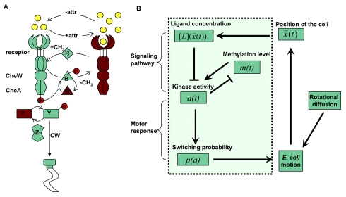
 . The internal signaling pathway dynamics is described at the coarse-grained level by the interactions between the average receptor methylation level
  and the kinase activity
  , which eventually determines the switching probability of the flagellar motor
  . The switching probability is then used to determine the cell motion (run or tumble), and direction of motion during run fluctuates due to rotational diffusion. The motion of the cell leads it to a new location with a new ligand concentration for the cell and the whole simulation process continues.
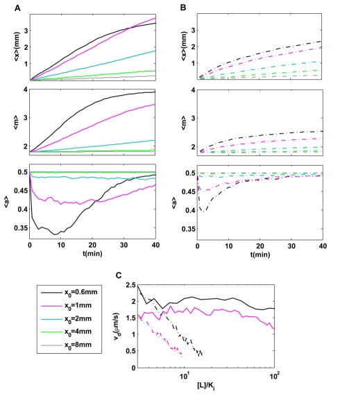
 . (B) Cell motion and intracellular dynamics in linear ligand profiles:
  . In both (A) & (B), the dynamics of the (population) averaged position (
 ); the average receptor methylation level (
 ) and the average kinase activity
  are shown for different decay lengths
  .
.  . The population-averaged position increases linearly with time until the methylation level reaches saturation in exponential profiles; while it slows down continuously in the linear profiles. After a transient decrease, the kinase activity stays roughly constant in exponential profiles, while it varies continuously recovering to its pre-stimulus level
  in linear profiles. (C) Direct comparison of instantaneous velocities between exponential (solid lines) and linear (dotted lines) profiles for
  (black); 1.0 mm (purple). Within the chemosensitivity range
  , the instantaneous chemotaxis drift velocity is constant in exponential profiles, while it decreases continuously with [L] in the linear ligand profiles.
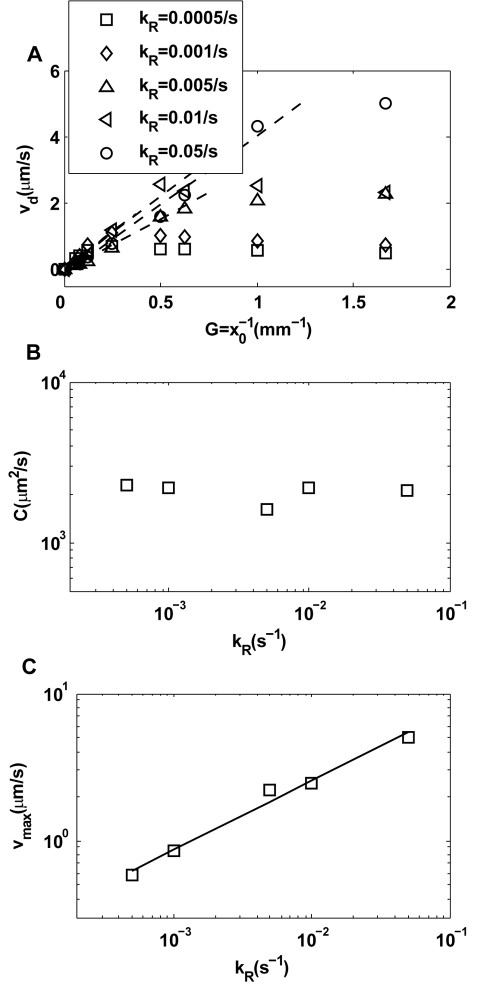
 for different exponential gradient
  . Different symbols represent different adaptation rates
  . Note that
  first increases linearly (dashed line) with
  before reaching a saturation velocity at a critical gradient
  ,. We can fit
  with:
with:  , in which
  is the chemotaxis motility constant given by the linear fitting coefficient and the saturation drift velocity is
  . The dependences of
  and
and  on
on  are shown in (B) and (C) respectively. For the range of
  we studied, we found that
  is roughly independent of
  and
and  depends on
  with a simple scaling relation:
  .
.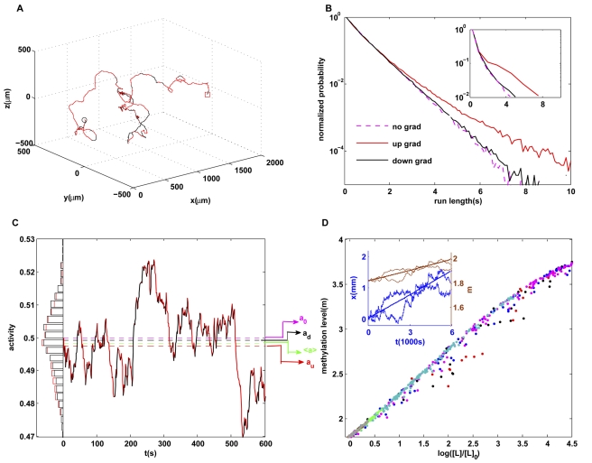
 with
with  . The random walk motion is biased towards the gradient (arrow). The forward runs up the gradient are in red, and the backward runs down the gradient are in black. (B) Run length distribution for forward runs (red), backward runs (black) in the presence of an exponential gradient and without a gradient (purple). The backward run length distribution is close to the run length distribution in the absence of a gradient, similar to the experimental results from Berg and Brown as reproduced in the inset. (C) Distributions of cell kinase activity for forward (red) and backward (black) runs. A time series of the activity
  of a single cell is shown: forward is in red and backward is in black. The average activity for backward (black dashed line) is closer to the adapted activity (purple dashed line, 0.5) compared with the average activity for forward (red dashed line). (D) Methylation level of different individual cells at different times and in different exponential gradients (represented by color symbols as in Figure 2) all increase with logarithmic ligand concentration along a universal line, despite large temporal fluctuations in methylation levels and positions for (two) individual cells as shown in the inset.
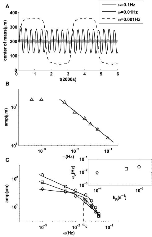
 ) is caused by boundary effects. (C) Upon decreasing adaptation rate, a transition to a steeper decay of the amplitude appears at frequencies higher than a transition frequency
  within the range of frequencies studied. Three cases with smaller values of
  are shown, and the dependence of
  on the adaptation rate
  is shown in the inset of (C).
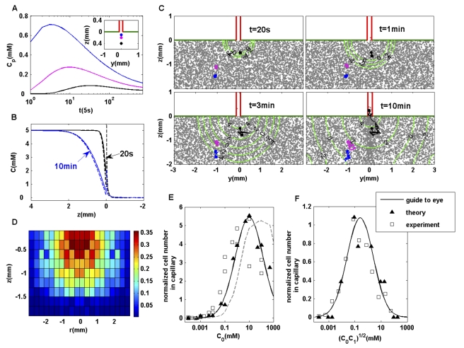
 . (B) The exact ligand profile (solid line) along the center line of the capillary at different times, in comparison with the asymptotic solutions (dashed lines) by Furtelle and Berg . (C) Cell density in the rectangular coordinate is shown together with the contours of the logarithmic ligand concentration (in
  ) at different times. Three individual cell trajectories (starting from circles and ending at squares) are shown. Only the black cell ends in the capillary. (D) Probability distribution of the original positions of cells that end in the capillary. For a cell originally located at position
  , the probability of it ending in the capillary at a later time (45 min),
  , is shown.
  ,
,  . (E) Concentration-response curve for the capillary assay. The average number of bacteria in the capillary after 45–50 min subtracted by the number of bacteria in the capillary in the absence of attractant is defined as the response (ordinate). The results from our model with the exact ligand profile are labeled by solid symbols (fitted by a solid line). They agree well with the experimental measurements (hollow squares) of Mesibov et al ,. The results from using the asymptotic ligand profile by Furtelle and Berg are shown by the dashed lines. (F) Response curve for capillary assay with
  . The solid symbols (fitted with a solid line) represent the model, and the hollow symbols represent the experimental results (both collected at 60 min).
Similar articles
-
Coarse graining Escherichia coli chemotaxis: from multi-flagella propulsion to logarithmic sensing.Adv Exp Med Biol. 2012;736:381-96. doi: 10.1007/978-1-4419-7210-1_22. Adv Exp Med Biol. 2012. PMID: 22161341
-
Logarithmic sensing in Escherichia coli bacterial chemotaxis.Biophys J. 2009 Mar 18;96(6):2439-48. doi: 10.1016/j.bpj.2008.10.027. Biophys J. 2009. PMID: 19289068 Free PMC article.
-
Mathematical modeling and experimental validation of chemotaxis under controlled gradients of methyl-aspartate in Escherichia coli.Mol Biosyst. 2010 Jun;6(6):1082-92. doi: 10.1039/b924368b. Epub 2010 Mar 18. Mol Biosyst. 2010. PMID: 20485750
-
Overview of mathematical approaches used to model bacterial chemotaxis I: the single cell.Bull Math Biol. 2008 Aug;70(6):1525-69. doi: 10.1007/s11538-008-9321-6. Epub 2008 Jul 19. Bull Math Biol. 2008. PMID: 18642048 Review.
-
Responding to chemical gradients: bacterial chemotaxis.Curr Opin Cell Biol. 2012 Apr;24(2):262-8. doi: 10.1016/j.ceb.2011.11.008. Epub 2011 Dec 9. Curr Opin Cell Biol. 2012. PMID: 22169400 Free PMC article. Review.
Cited by
-
A new mode of swimming in singly flagellated Pseudomonas aeruginosa.Proc Natl Acad Sci U S A. 2022 Apr 5;119(14):e2120508119. doi: 10.1073/pnas.2120508119. Epub 2022 Mar 29. Proc Natl Acad Sci U S A. 2022. PMID: 35349348 Free PMC article.
-
Collective motion enhances chemotaxis in a two-dimensional bacterial swarm.Biophys J. 2021 May 4;120(9):1615-1624. doi: 10.1016/j.bpj.2021.02.021. Epub 2021 Feb 23. Biophys J. 2021. PMID: 33636168 Free PMC article.
-
Individual-Based Modeling of Spatial Dynamics of Chemotactic Microbial Populations.ACS Synth Biol. 2022 Nov 18;11(11):3714-3723. doi: 10.1021/acssynbio.2c00322. Epub 2022 Nov 6. ACS Synth Biol. 2022. PMID: 36336839 Free PMC article.
-
Noise-Induced Increase of Sensitivity in Bacterial Chemotaxis.Biophys J. 2016 Jul 26;111(2):430-437. doi: 10.1016/j.bpj.2016.06.013. Biophys J. 2016. PMID: 27463144 Free PMC article.
-
Physical limits on bacterial navigation in dynamic environments.J R Soc Interface. 2016 Jan;13(114):20150844. doi: 10.1098/rsif.2015.0844. J R Soc Interface. 2016. PMID: 26763331 Free PMC article.
References
-
- Sourjik V. Receptor clustering and signal processing in E.coli chemotaxis. Trends Microbiol. 2004;12:569–576. - PubMed
-
- Stock J, Re SD. In: Chemotaxis. Lederberg J, Alexander M, Bloom B, Hopwood D, Hull R, editors. San Diego, CA: Academic Press; 2000. pp. 772–780.
Publication types
MeSH terms
Grants and funding
LinkOut - more resources
Full Text Sources
Miscellaneous
