. 2010 May;255(2):442-50.
doi: 10.1148/radiol.10090281.

Sentinel lymph nodes and lymphatic vessels: noninvasive dual-modality in vivo mapping by using indocyanine green in rats--volumetric spectroscopic photoacoustic imaging and planar fluorescence imaging

Affiliations

Sentinel lymph nodes and lymphatic vessels: noninvasive dual-modality in vivo mapping by using indocyanine green in rats--volumetric spectroscopic photoacoustic imaging and planar fluorescence imaging

Chulhong Kim et al. Radiology. 2010 May.

Abstract

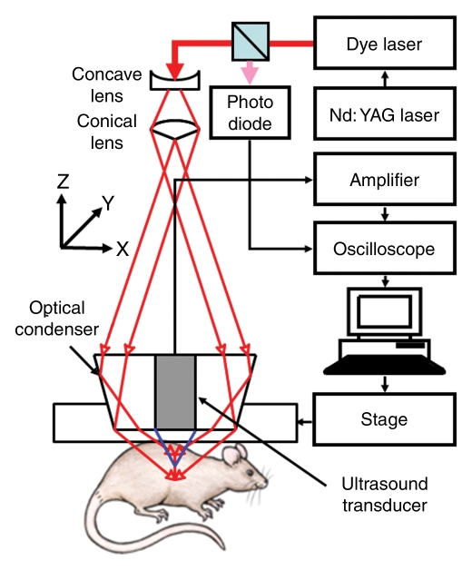
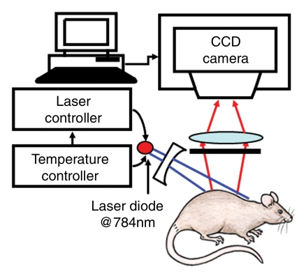
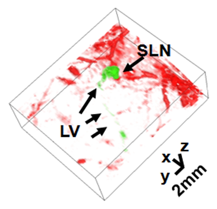
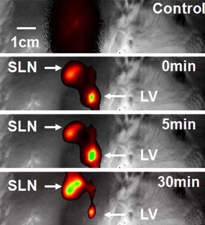
Purpose: To noninvasively map sentinel lymph nodes (SLNs) and lymphatic vessels in rats in vivo by using dual-modality nonionizing imaging-volumetric spectroscopic photoacoustic imaging, which measures optical absorption, and planar fluorescence imaging, which measures fluorescent emission-of indocyanine green (ICG).

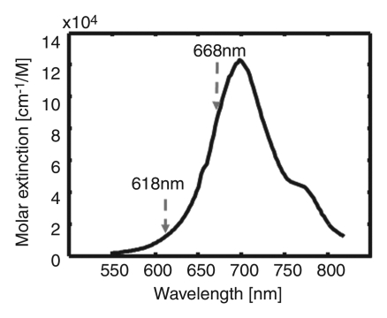
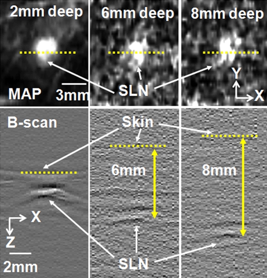
Materials and methods: Institutional animal care and use committee approval was obtained. Healthy Sprague-Dawley rats weighing 250-420 g (age range, 60-120 days) were imaged by using volumetric photoacoustic imaging (n = 5) and planar fluorescence imaging (n = 3) before and after injection of 1 mmol/L ICG. Student paired t tests based on a logarithmic scale were performed to evaluate the change in photoacoustic signal enhancement of SLNs and lymphatic vessels before and after ICG injection. The spatial resolutions of both imaging systems were compared at various imaging depths (2-8 mm) by layering additional biologic tissues on top of the rats in vivo. Spectroscopic photoacoustic imaging was applied to identify ICG-dyed SLNs.

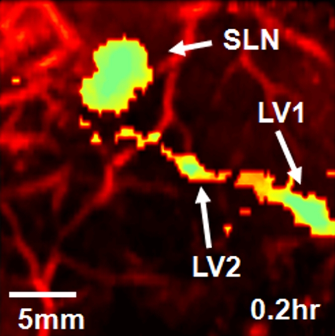
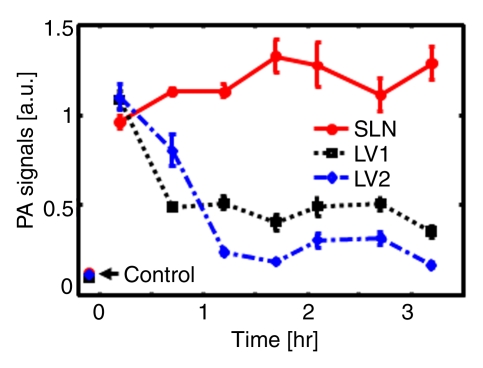
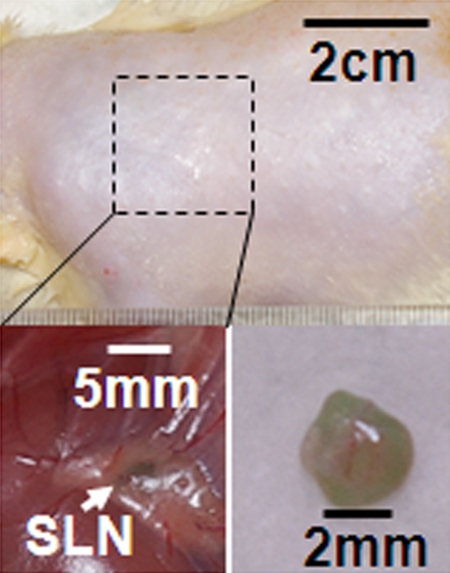
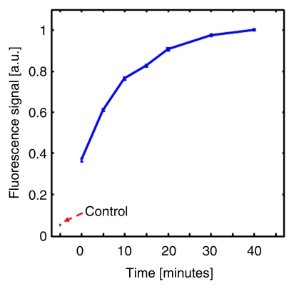
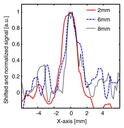
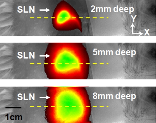
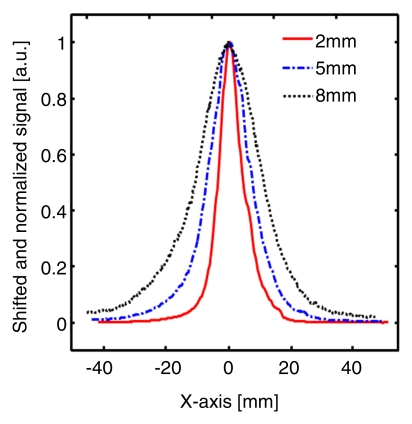
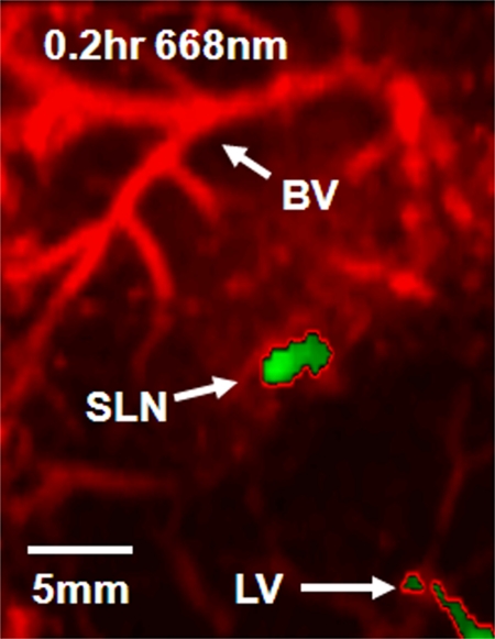
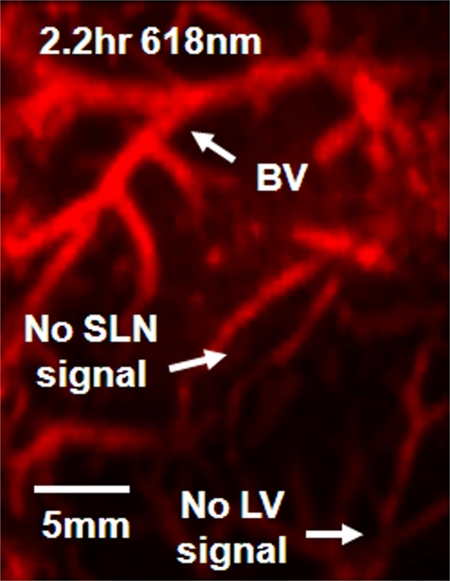
Results: In all five rats examined with photoacoustic imaging, SLNs were clearly visible, with a mean signal enhancement of 5.9 arbitrary units (AU) + or - 1.8 (standard error of the mean) (P < .002) at 0.2 hour after injection, while lymphatic vessels were seen in four of the five rats, with a signal enhancement of 4.3 AU + or - 0.6 (P = .001). In all three rats examined with fluorescence imaging, SLNs and lymphatic vessels were seen. The average full width at half maximum (FWHM) of the SLNs in the photoacoustic images at three imaging depths (2, 6, and 8 mm) was 2.0 mm + or - 0.2 (standard deviation), comparable to the size of a dissected lymph node as measured with a caliper. However, the FWHM of the SLNs in fluorescence images widened from 8 to 22 mm as the imaging depth increased, owing to strong light scattering. SLNs were identified spectroscopically in photoacoustic images.

Conclusion: These two modalities, when used together with ICG, have the potential to help map SLNs in axillary staging and to help evaluate tumor metastasis in patients with breast cancer.


Figures

Figure 1a:
Figure 1a:
(a) Experimental setup of the photoacoustic imaging system. (b) Experimental setup of the fluorescence imaging system. CCD = charge-coupled device. (c) Optical spectrum of 1 mmol/L ICG. A wavelength of 668 nm was used for photoacoustic imaging experiments. For spectroscopic photoacoustic imaging, wavelengths of 618 and 668 nm were chosen.
Figure 1b:
Figure 1b:
(a) Experimental setup of the photoacoustic imaging system. (b) Experimental setup of the fluorescence imaging system. CCD = charge-coupled device. (c) Optical spectrum of 1 mmol/L ICG. A wavelength of 668 nm was used for photoacoustic imaging experiments. For spectroscopic photoacoustic imaging, wavelengths of 618 and 668 nm were chosen.
Figure 1c:
Figure 1c:
(a) Experimental setup of the photoacoustic imaging system. (b) Experimental setup of the fluorescence imaging system. CCD = charge-coupled device. (c) Optical spectrum of 1 mmol/L ICG. A wavelength of 668 nm was used for photoacoustic imaging experiments. For spectroscopic photoacoustic imaging, wavelengths of 618 and 668 nm were chosen.
Figure 2a:
Figure 2a:
Volumetric photoacoustic imaging. (a) Control MAP image acquired before ICG injection in the axillary region. Blood vessels (BV) are seen. (b) Photoacoustic image acquired 0.2 hour after injection. Lymphatic vessels, as well as an SLN, are seen. (c) Three-dimensional photoacoustic image processed from the 0.7-hour postinjection data shown in Figure E1 (online). (d) Graph shows results of comparison of photoacoustic (PA) signals within the SLN and lymphatic vessels (LV) versus time before and after the injection in a given rat. The photoacoustic signals were normalized by the photoacoustic signals of adjacent blood vessels. (e) Graph shows results of statistical comparison of photoacoustic signal enhancement in the background (BG) (n = 5), SLN (n = 5), and lymphatic vessels (n = 4) at 0.2 and 1 hour after injection. The P values for the SLN and lymphatic vessels, respectively, were less than .002 and .001 at 0.2 hour after injection and less than .001 and .13 at 1 hour after injection. (f) Photographs of rat before dissection (top), axillary region after dissection (bottom left), and ICG-dyed lymph node (bottom right). a.u. = Arbitrary units (AU), error bars in d = standard deviation, error bars in e = standard error of the mean.
Figure 2b:
Figure 2b:
Volumetric photoacoustic imaging. (a) Control MAP image acquired before ICG injection in the axillary region. Blood vessels (BV) are seen. (b) Photoacoustic image acquired 0.2 hour after injection. Lymphatic vessels, as well as an SLN, are seen. (c) Three-dimensional photoacoustic image processed from the 0.7-hour postinjection data shown in Figure E1 (online). (d) Graph shows results of comparison of photoacoustic (PA) signals within the SLN and lymphatic vessels (LV) versus time before and after the injection in a given rat. The photoacoustic signals were normalized by the photoacoustic signals of adjacent blood vessels. (e) Graph shows results of statistical comparison of photoacoustic signal enhancement in the background (BG) (n = 5), SLN (n = 5), and lymphatic vessels (n = 4) at 0.2 and 1 hour after injection. The P values for the SLN and lymphatic vessels, respectively, were less than .002 and .001 at 0.2 hour after injection and less than .001 and .13 at 1 hour after injection. (f) Photographs of rat before dissection (top), axillary region after dissection (bottom left), and ICG-dyed lymph node (bottom right). a.u. = Arbitrary units (AU), error bars in d = standard deviation, error bars in e = standard error of the mean.
Figure 2c:
Figure 2c:
Volumetric photoacoustic imaging. (a) Control MAP image acquired before ICG injection in the axillary region. Blood vessels (BV) are seen. (b) Photoacoustic image acquired 0.2 hour after injection. Lymphatic vessels, as well as an SLN, are seen. (c) Three-dimensional photoacoustic image processed from the 0.7-hour postinjection data shown in Figure E1 (online). (d) Graph shows results of comparison of photoacoustic (PA) signals within the SLN and lymphatic vessels (LV) versus time before and after the injection in a given rat. The photoacoustic signals were normalized by the photoacoustic signals of adjacent blood vessels. (e) Graph shows results of statistical comparison of photoacoustic signal enhancement in the background (BG) (n = 5), SLN (n = 5), and lymphatic vessels (n = 4) at 0.2 and 1 hour after injection. The P values for the SLN and lymphatic vessels, respectively, were less than .002 and .001 at 0.2 hour after injection and less than .001 and .13 at 1 hour after injection. (f) Photographs of rat before dissection (top), axillary region after dissection (bottom left), and ICG-dyed lymph node (bottom right). a.u. = Arbitrary units (AU), error bars in d = standard deviation, error bars in e = standard error of the mean.
Figure 2d:
Figure 2d:
Volumetric photoacoustic imaging. (a) Control MAP image acquired before ICG injection in the axillary region. Blood vessels (BV) are seen. (b) Photoacoustic image acquired 0.2 hour after injection. Lymphatic vessels, as well as an SLN, are seen. (c) Three-dimensional photoacoustic image processed from the 0.7-hour postinjection data shown in Figure E1 (online). (d) Graph shows results of comparison of photoacoustic (PA) signals within the SLN and lymphatic vessels (LV) versus time before and after the injection in a given rat. The photoacoustic signals were normalized by the photoacoustic signals of adjacent blood vessels. (e) Graph shows results of statistical comparison of photoacoustic signal enhancement in the background (BG) (n = 5), SLN (n = 5), and lymphatic vessels (n = 4) at 0.2 and 1 hour after injection. The P values for the SLN and lymphatic vessels, respectively, were less than .002 and .001 at 0.2 hour after injection and less than .001 and .13 at 1 hour after injection. (f) Photographs of rat before dissection (top), axillary region after dissection (bottom left), and ICG-dyed lymph node (bottom right). a.u. = Arbitrary units (AU), error bars in d = standard deviation, error bars in e = standard error of the mean.
Figure 2e:
Figure 2e:
Volumetric photoacoustic imaging. (a) Control MAP image acquired before ICG injection in the axillary region. Blood vessels (BV) are seen. (b) Photoacoustic image acquired 0.2 hour after injection. Lymphatic vessels, as well as an SLN, are seen. (c) Three-dimensional photoacoustic image processed from the 0.7-hour postinjection data shown in Figure E1 (online). (d) Graph shows results of comparison of photoacoustic (PA) signals within the SLN and lymphatic vessels (LV) versus time before and after the injection in a given rat. The photoacoustic signals were normalized by the photoacoustic signals of adjacent blood vessels. (e) Graph shows results of statistical comparison of photoacoustic signal enhancement in the background (BG) (n = 5), SLN (n = 5), and lymphatic vessels (n = 4) at 0.2 and 1 hour after injection. The P values for the SLN and lymphatic vessels, respectively, were less than .002 and .001 at 0.2 hour after injection and less than .001 and .13 at 1 hour after injection. (f) Photographs of rat before dissection (top), axillary region after dissection (bottom left), and ICG-dyed lymph node (bottom right). a.u. = Arbitrary units (AU), error bars in d = standard deviation, error bars in e = standard error of the mean.
Figure 2f:
Figure 2f:
Volumetric photoacoustic imaging. (a) Control MAP image acquired before ICG injection in the axillary region. Blood vessels (BV) are seen. (b) Photoacoustic image acquired 0.2 hour after injection. Lymphatic vessels, as well as an SLN, are seen. (c) Three-dimensional photoacoustic image processed from the 0.7-hour postinjection data shown in Figure E1 (online). (d) Graph shows results of comparison of photoacoustic (PA) signals within the SLN and lymphatic vessels (LV) versus time before and after the injection in a given rat. The photoacoustic signals were normalized by the photoacoustic signals of adjacent blood vessels. (e) Graph shows results of statistical comparison of photoacoustic signal enhancement in the background (BG) (n = 5), SLN (n = 5), and lymphatic vessels (n = 4) at 0.2 and 1 hour after injection. The P values for the SLN and lymphatic vessels, respectively, were less than .002 and .001 at 0.2 hour after injection and less than .001 and .13 at 1 hour after injection. (f) Photographs of rat before dissection (top), axillary region after dissection (bottom left), and ICG-dyed lymph node (bottom right). a.u. = Arbitrary units (AU), error bars in d = standard deviation, error bars in e = standard error of the mean.
Figure 3a:
Figure 3a:
(a) Coronal planar fluorescence images acquired before injection (Control) and 0, 5, and 30 minutes after injection of ICG in a rat. LV = lymphatic vessel. (b) Bar graph shows changes in fluorescence signals within the SLN region after the injection.
Figure 3b:
Figure 3b:
(a) Coronal planar fluorescence images acquired before injection (Control) and 0, 5, and 30 minutes after injection of ICG in a rat. LV = lymphatic vessel. (b) Bar graph shows changes in fluorescence signals within the SLN region after the injection.
Figure 4a:
Figure 4a:
Comparison of spatial resolutions between photoacoustic and fluorescence images with increases in imaging depth increments. (a) Photoacoustic MAP (top row) and corresponding depth-resolved B-scan (bottom row) images of SLNs at three depths. (b) Graph shows results for three 1D profiles taken from along the dotted lines in the MAP images in a. (c) Fluorescence images of SLNs at three depths. (d) Graph shows results for three 1D profiles taken from along the dashed lines in c.
Figure 4b:
Figure 4b:
Comparison of spatial resolutions between photoacoustic and fluorescence images with increases in imaging depth increments. (a) Photoacoustic MAP (top row) and corresponding depth-resolved B-scan (bottom row) images of SLNs at three depths. (b) Graph shows results for three 1D profiles taken from along the dotted lines in the MAP images in a. (c) Fluorescence images of SLNs at three depths. (d) Graph shows results for three 1D profiles taken from along the dashed lines in c.
Figure 4c:
Figure 4c:
Comparison of spatial resolutions between photoacoustic and fluorescence images with increases in imaging depth increments. (a) Photoacoustic MAP (top row) and corresponding depth-resolved B-scan (bottom row) images of SLNs at three depths. (b) Graph shows results for three 1D profiles taken from along the dotted lines in the MAP images in a. (c) Fluorescence images of SLNs at three depths. (d) Graph shows results for three 1D profiles taken from along the dashed lines in c.
Figure 4d:
Figure 4d:
Comparison of spatial resolutions between photoacoustic and fluorescence images with increases in imaging depth increments. (a) Photoacoustic MAP (top row) and corresponding depth-resolved B-scan (bottom row) images of SLNs at three depths. (b) Graph shows results for three 1D profiles taken from along the dotted lines in the MAP images in a. (c) Fluorescence images of SLNs at three depths. (d) Graph shows results for three 1D profiles taken from along the dashed lines in c.
Figure 5a:
Figure 5a:
Spectroscopic photoacoustic images. (a) Image at 668 nm 0.2 hour after injection. (b) Image at 618 nm 2.2 hours after injection. (c) Image at 668 nm 2.8 hours after injection. (d) Graph shows comparison of spectroscopic photoacoustic (PA) signals within the SLN region over a period of time. (e) Graph shows comparison of spectroscopic photoacoustic signals within blood vessels (BV) over a period of time. LV = lymphatic vessel. Numbers in colored bar at top of d and e = wavelength in nanometers.
Figure 5b:
Figure 5b:
Spectroscopic photoacoustic images. (a) Image at 668 nm 0.2 hour after injection. (b) Image at 618 nm 2.2 hours after injection. (c) Image at 668 nm 2.8 hours after injection. (d) Graph shows comparison of spectroscopic photoacoustic (PA) signals within the SLN region over a period of time. (e) Graph shows comparison of spectroscopic photoacoustic signals within blood vessels (BV) over a period of time. LV = lymphatic vessel. Numbers in colored bar at top of d and e = wavelength in nanometers.
Figure 5c:
Figure 5c:
Spectroscopic photoacoustic images. (a) Image at 668 nm 0.2 hour after injection. (b) Image at 618 nm 2.2 hours after injection. (c) Image at 668 nm 2.8 hours after injection. (d) Graph shows comparison of spectroscopic photoacoustic (PA) signals within the SLN region over a period of time. (e) Graph shows comparison of spectroscopic photoacoustic signals within blood vessels (BV) over a period of time. LV = lymphatic vessel. Numbers in colored bar at top of d and e = wavelength in nanometers.
Figure 5d:
Figure 5d:
Spectroscopic photoacoustic images. (a) Image at 668 nm 0.2 hour after injection. (b) Image at 618 nm 2.2 hours after injection. (c) Image at 668 nm 2.8 hours after injection. (d) Graph shows comparison of spectroscopic photoacoustic (PA) signals within the SLN region over a period of time. (e) Graph shows comparison of spectroscopic photoacoustic signals within blood vessels (BV) over a period of time. LV = lymphatic vessel. Numbers in colored bar at top of d and e = wavelength in nanometers.
Figure 5e:
Figure 5e:
Spectroscopic photoacoustic images. (a) Image at 668 nm 0.2 hour after injection. (b) Image at 618 nm 2.2 hours after injection. (c) Image at 668 nm 2.8 hours after injection. (d) Graph shows comparison of spectroscopic photoacoustic (PA) signals within the SLN region over a period of time. (e) Graph shows comparison of spectroscopic photoacoustic signals within blood vessels (BV) over a period of time. LV = lymphatic vessel. Numbers in colored bar at top of d and e = wavelength in nanometers.

References

    1. Kobayashi H, Kawamoto S, Sakai Y, et al. Lymphatic drainage imaging of breast cancer in mice by micro-magnetic resonance lymphangiography using a nano-size paramagnetic contrast agent. J Natl Cancer Inst 2004;96(9):703–708 - PubMed
    1. McMasters KM, Tuttle TM, Carlson DJ, et al. Sentinel lymph node biopsy for breast cancer: a suitable alternative to routine axillary dissection in multi-institutional practice when optimal technique is used. J Clin Oncol 2000;18(13):2560–2566 - PubMed
    1. Ung OA. Australasian experience and trials in sentinel lymph node biopsy: the RACS SNAC trial. Asian J Surg 2004;27(4):284–290 - PubMed
    1. Purushotham AD, Upponi S, Klevesath MB, et al. Morbidity after sentinel lymph node biopsy in primary breast cancer: results from a randomized controlled trial. J Clin Oncol 2005;23(19):4312–4321 - PubMed
    1. Krishnamurthy S, Sneige N, Bedi DG, et al. Role of ultrasound-guided fine-needle aspiration of indeterminate and suspicious axillary lymph nodes in the initial staging of breast carcinoma. Cancer 2002;95(5):982–988 - PubMed