What role does natural selection play in speciation?

Abstract

If distinct biological species are to coexist in sympatry, they must be reproductively isolated and must exploit different limiting resources. A two-niche Levene model is analysed, in which habitat preference and survival depend on underlying additive traits. The population genetics of preference and viability are equivalent. However, there is a linear trade-off between the chances of settling in either niche, whereas viabilities may be constrained arbitrarily. With a convex trade-off, a sexual population evolves a single generalist genotype, whereas with a concave trade-off, disruptive selection favours maximal variance. A pure habitat preference evolves to global linkage equilibrium if mating occurs in a single pool, but remarkably, evolves to pairwise linkage equilibrium within niches if mating is within those niches--independent of the genetics. With a concave trade-off, the population shifts sharply between a unimodal distribution with high gene flow and a bimodal distribution with strong isolation, as the underlying genetic variance increases. However, these alternative states are only simultaneously stable for a narrow parameter range. A sharp threshold is only seen if survival in the 'wrong' niche is low; otherwise, strong isolation is impossible. Gene flow from divergent demes makes speciation much easier in parapatry than in sympatry.

Figure 1.

(a) Mutations A and B arise in one lineage, and C and D in another. The descendant populations have genotype ABcd and abCD, and are separated by two Dobzhansky-Muller incompatibilities (DMIs), indicated by thin lines: allele A is incompatible with D, and B with C. Both incompatibilities are between two derived alleles. (b) If the ancestral genotype were ABcd, and four mutations occurred in one lineage (B → b, A → a, c → C, d → D), then the descendant populations would have the same genotypes, but both incompatibilities would be between a derived and an ancestral allele. All that has changed is the position of the root.

Figure 2.

DMIs can accumulate in parapatry as well as in allopatry. (a) Alleles A and D arise at different places, and at different loci, and both begin to spread. (b) If they meet, and are incompatible, then they will remain separated by a stable pair of clines (double lines). New alleles may then arise (B,C); if these are incompatible with each other, or with one of the alleles that are already established, then they will strengthen the isolation, leading to a set of four clines.

Figure 3.

The distribution of viability, v₁, caused by a normal distribution of the underlying trait, z. This changes from unimodal through to bimodal as the variance in z increases from 0.1 to 1 to 10; mean z = 1, β = 2.

Figure 4.

(a) The possible viabilities in each niche are limited by a trade-off curve (equation (2.3)). For β = 1, there is a linear trade-off (v₀ + v₁ ≤ 1; middle line), and any distribution on this line that has mean v̄ = 1 is an ESS. For β = 0.5, the trade-off curve is convex (upper curve), and there is a unique monomorphic ESS for viability (shown at upper right, for c₀ = c₁ = 0.5). Conversely, for β = 2, the trade-off curve is concave, and there is a unique polymorphic ESS, with a mixture of specialist genotypes (dots at upper left, lower right). (b) If both preference and viability vary, and if there is no recombination between them, then what matters is the constraint on the product α_γv_γ. The curves here show the combined trade-off (equation (2.5)) for the viabilities shown in (a), and habitat preference (α₀ + α₁ = 1; equation (2.4)). These are concave, for all β, and so the ESS is always for a polymorphism between two extreme specialists (dots).

Figure 5.

The trade-off curve is the outer limit of the set of possible viabilities, {v₀, v₁}: it does not require that mutations have effects that fall on this curve. To illustrate this point, the distribution of genotypic values is shown, for viabilities determined by underlying additive traits {z₀, z₁} (equation (2.2)). These traits are determined as the sum of random effects at 10 loci, with effects on z₀, z₁ at each locus chosen independently from a random uniform distribution, but with the constraint that z₀ + z₁ ≤ 2 log (β); here, β = 2. Selection will take the population close to the trade-off curve.

Figure 6.

When constraints on preference (α₀ + α₁ = 1) and viability (v₀, v₁) are combined, the trade-off curve for net fitness (α₀v₀, α₁v₁) is always concave. Therefore, in an asexual population, the ESS is always for polymorphism between two extreme specialists, if preference and viability can evolve together. (a) The constraint on viability (equation (2.4)) is convex, straight or concave, depending on whether β = 0.5, 1 or 2 (top right to lower left). (b) The corresponding constraint on net fitness (α_γv_γ) is always concave (θ = 0.1 throughout).

Figure 7.

(a) The equilibrium viabilities in the two niches, plotted against the size of niche 1, c₁; β = 2, θ = 0. There is a single intermediate equilibrium, which smoothly tracks niche size. (b) With θ = 0.1, populations specialize on the commonest niche when that niche predominates (c₁/c₀ < β²θ, c₁/c₀ > 1/β²θ or c₁ < 0.29, c₁ > 0.71); however, for intermediate c₁, there is an intermediate equilibrium, as in (a). (c) With θ = 0.4, there is an intermediate region with two stable equilibria (0.38 < c₁ < 0.62). If these meet in a cline, a narrow tension zone will form, centred on z = 0 (dashed line). (Only the mean viability in niche 1 is shown here, for clarity.)

Figure 8.

The probability that a surviving parent in one niche was born in a different niche, plotted against the within-niche variance in underlying preference, var(a). Solid line: symmetric case, c₀ = c₁ = 0.5; dashed lines: asymmetric case, c₀ = 0.2, c₁ = 0.8. The upper dashed line shows the chance that a parent in the smaller niche came from elsewhere, and the lower dashed line, the chance that a parent in the larger niche came from elsewhere. The long dashed line at the centre shows the weighted average of these two. This assumes the infinitesimal model, which has a Gaussian solution (equation (4.2)).

Figure 9.

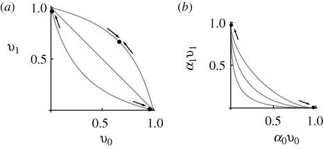
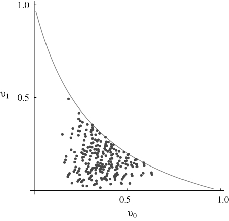
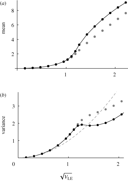
The mean and variance within niches, plotted against the standard deviation at linkage equilibrium, . The dots connected by a solid line show the exact solution, obtained by iterating until convergence. (Starting from linkage equilibrium, and from complete disequilibrium, led to the same values.) Grey dots show the Gaussian approximation. The dashed line in (b) shows the variance at linkage equilibrium, in the population as a whole. There are n = 40 loci, and equal niche sizes; β = 2; values are measured in the newborn population.

Figure 10.

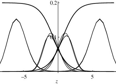
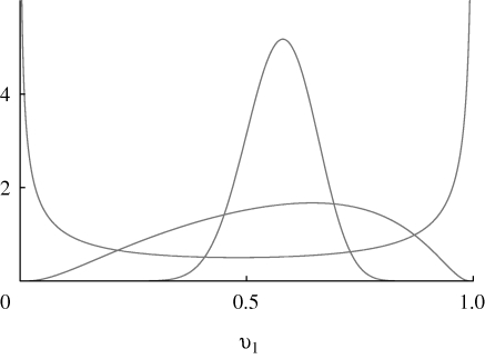
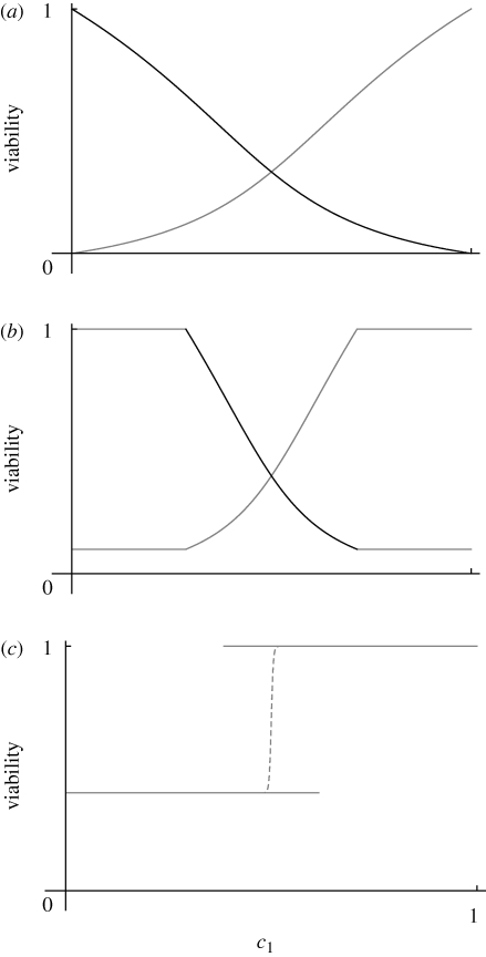
The distributions of the trait, z, within each of the two niches, for standard deviation = 0.95 (inner pair) and 1.6 (outer pair); these correspond to allelic effects Z = 0.3, 0.5, respectively. The upper pair of logistic curves show how the viabilities depend on z. For (outer pair), the distributions before and after reproduction are indistinguishable, implying linkage equilibrium. However, for smaller allelic effects (inner pair), there is appreciable linkage disequilibrium; the solid lines show the distribution within niches immediately before reproduction, and the thin lines, the distribution amongst newborns. Parameters as in figure 9.

Figure 11.

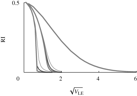
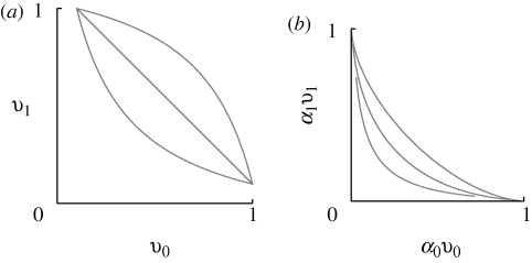
The chance that a survivor in one niche was born in a different niche, plotted against the standard deviation at linkage equilibrium , assuming equal allele frequencies. Each set of curves is for β = 1, 2, 4 (right to left); within each set, the three curves are for n = 10, 20, 40 loci (thin to thick lines). Otherwise, parameters as in figure 9.

Figure 12.

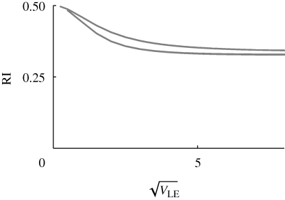
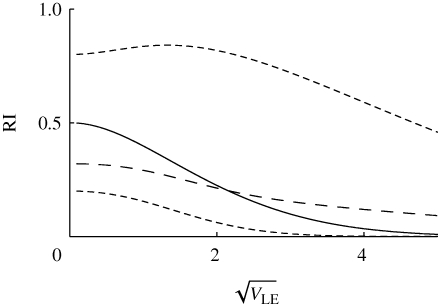
Reproductive isolation, given that there is a minimum survival θ = 0.2 in the unsuitable niche (equation (2.4)). As in figure 11, this shows the chance that a survivor in one niche was born in a different niche, plotted against . Results for n = 10, 20, 40 loci are indistinguishable. The two curves are for β = 1 (top) and β = 2 (bottom); for = 2.2, the population fixes for one or other specialist.

Figure 13.

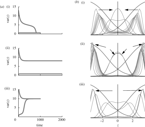
Behaviour near the threshold between unimodal and bimodal equilibria. (a) Shows the trait variance, across both niches, against time, starting either from complete linkage disequilibrium (LD, a(i)) or linkage equilibrium (LE, a(iii)). There are n = 40 loci, β = 4, and niches are of equal size. The standard deviation at linkage equilibrium is (a)(i)–(iii). (b) Shows the viabilities in each niche (thick curves; equation (2.3)), together with the trait distribution over successive generations. (i) , t = 100, 200, … , 1000, starting in LD; (ii) , t = 20, 40, … , 200, starting in LD and in LE; (iii) , t = 100, 200, … , 1000, starting in LE.

Figure 14.

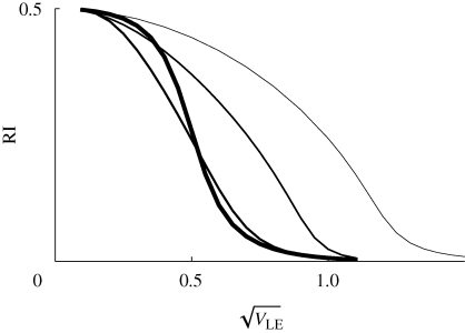
The effect of migration, m, on reproductive isolation. The chance that a survivor in one niche was born in a different niche (RI) is plotted against the standard deviation at linkage equilibrium , as in figure 11. Migration rate is m = 0, 0.02, 0.1, 0.5 (thin to thick lines). The focal deme exchanges a fraction m/2 of individuals with each of two flanking demes; one has only niche 0, and the other, only niche 1. β = 2, n = 40 loci; otherwise, parameters as in figure 9.

Figure 15.

Effect of gene flow across a linear cline. Niche size, c₁, changes across a cline of 40 demes, in a logistic curve with width (defines as 1/max. gradient) plotted on the horizontal axis. (a) Shows the chance that an individual niche 1 in the central deme was born in niche 0 (regardless of spatial location). (b) Shows the width of the cline in trait mean; the dashed curve indicates the line where the two widths are equal. 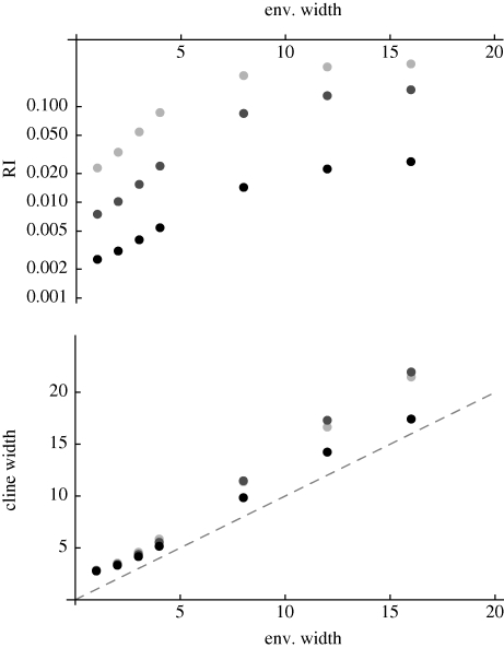β = 2, θ = 0, 20 loci; (black to light grey).

Figure 16.

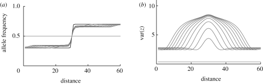
Speciation can be triggered by gene flow in parapatry. In this example, selection is in the narrow range in which alternative stable states are possible: β = 4, θ = 0, 0, n = 40 loci (figure 13, a(ii), b(ii)). The population is distributed on a linear cline of 60 demes, with migration between nearest neighbours at a rate m = 1/2; niche size varies along the cline, from 0.3 on the left to 0.7 on the right, in a logistic curve with width 1 (black curve at (a)). Initially, the population is at linkage equilibrium with equal allele frequencies. (a) Shows the allele frequency clines at t = 0, 200, … , 2000 generations; (b) shows the clines in trait variance, over the same intervals.

References

-
- Barton N. H., de Cara M. A. R.2009The evolution of strong reproductive isolation. Evolution 63, 1171–1190 (doi:10.1111/j.1558-5646.2009.00622.x) - DOI - PubMed
- Barton N. H., Shpak M.2000The stability of symmetrical solutions to polygenic models. Theor. Popul. Biol. 57, 249–264 (doi:10.1006/tpbi.2000.1455) - DOI - PubMed
- Bateson W.1909Heredity and variation in modern lights. In Darwin and modern science (ed. Seward A. C.), pp. 85–101 Cambridge, UK: Cambridge University Press
- Bomblies K., Weigel D.2010Arabidopsis and relatives as models for the study of genetic and genomic incompatibilities. Phil. Trans. R. Soc. B 365, 1815–1823 (doi:10.1098/rstb.2009.0304) - DOI - PMC - PubMed
Publication types
MeSH terms
LinkOut - more resources
Full Text Sources