A critical quantity for noise attenuation in feedback systems

Abstract

Feedback modules, which appear ubiquitously in biological regulations, are often subject to disturbances from the input, leading to fluctuations in the output. Thus, the question becomes how a feedback system can produce a faithful response with a noisy input. We employed multiple time scale analysis, Fluctuation Dissipation Theorem, linear stability, and numerical simulations to investigate a module with one positive feedback loop driven by an external stimulus, and we obtained a critical quantity in noise attenuation, termed as "signed activation time". We then studied the signed activation time for a system of two positive feedback loops, a system of one positive feedback loop and one negative feedback loop, and six other existing biological models consisting of multiple components along with positive and negative feedback loops. An inverse relationship is found between the noise amplification rate and the signed activation time, defined as the difference between the deactivation and activation time scales of the noise-free system, normalized by the frequency of noises presented in the input. Thus, the combination of fast activation and slow deactivation provides the best noise attenuation, and it can be attained in a single positive feedback loop system. An additional positive feedback loop often leads to a marked decrease in activation time, decrease or slight increase of deactivation time and allows larger kinetic rate variations for slow deactivation and fast activation. On the other hand, a negative feedback loop may increase the activation and deactivation times. The negative relationship between the noise amplification rate and the signed activation time also holds for the six other biological models with multiple components and feedback loops. This principle may be applicable to other feedback systems.

Figure 1. Schematic diagrams of single-positive-loop, positive-positive-loop, and positive-negative-loop modules.

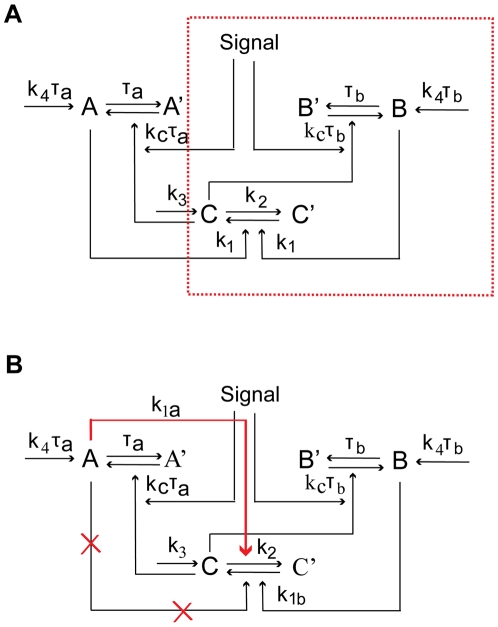
(A) The positive feedback modules. In this plot, there are three components: loop , loop , and output . , , and denote the active forms, whereas , , and stand for the corresponding inactive forms, respectively. The red dashed box represents the single-positive-loop module consisting of and only. In the component, signals come in to active with the help of at the rate of . All other activation processes of are lumped into one term, the basal activation rate . The conversion from to has the rate . In the component, is activated by at the rate of , and the deactivation of is at the rate of . The basal activation rate of is . Similar notations are used in the component. (B) The positive-negative-loop module. The positive feedback from to is replaced by negative feedback (red arrow).

Figure 2. Schematic illustration of the activation (left) and deactivation (right) time scales.

Figure 3. Noise attenuation and time scales in single-positive-loop systems.

(A) A noisy signal with frequency and (defined in Methods). (B) A typical output response to the signal in (A). (C) versus . Kinetic parameters (black), (red), (green), and (blue) are varied individually to tune and while is fixed. The curve (black): , ; the curve (red): , ; the curve (green): , ; the curve (blue): , . (D) Four sets of kinetic parameters are chosen, and each set corresponds to one curve. On each curve, is varied, and the kinetic parameters are fixed. Each point represents an average of based on simulations with different noisy signals but fixed . Set (blue): , , . Set (black): , , . Set (red): , , . Set (green): , , . In set , takes , . For the rest, , . (E) (bottom) and (top) versus . Parameters are the same as the corresponding color set in (D). , . (F) (bottom) and (top) versus . (set 1, blue), (set 2, red). In each plot, , . In all simulations, , , , unless otherwise specified.

Figure 4. Noise attenuation and time scales in positive-positive-loop systems.

(A–B) The same plots as in Figures 3C–3D but with the additional positive feedback loop , where . (C–D) The change of (bottom) and (top) with respect to (C) and (D) in single-positive-loop (blue), fast-slow-loop (, black), and slow-slow-loop (, red) systems. and are varied the same way as in Figure 3E and Figure 3F, respectively. (E–F) The ratio of in positive-positive-loop systems to in the corresponding single-positive-loop systems with respect to (E) and (F). (blue), (black), and (red). All simulations use the same parameters and inputs as their counterparts in Figure 3 with the additional parameter , unless otherwise specified.

Figure 5. Noise attenuation and time scales in positive-negative-loop systems.

(A) Kinetic parameters (black), (orange), (red), (green), (purple), (cyan), and (blue) are varied individually to tune and while is fixed. In each parameter variation, samples are simulated. (B) The dependence of on when is varied and the kinetic parameters are fixed. We use the same four sets of parameters as in Figure 3D with the additional parameters . (C–D) The change of (bottom) and (top) with respect to (C) and (D) in single-positive-loop (blue), positive-negative-loop (, black), and positive-negative-loop (, red) systems. and are varied the same way as in Figure 3E and Figure 3F, respectively.

Figure 6. Noise attenuation in a yeast cell polarization model.

(A) Schematic diagram of the yeast cell polarization signal transduction pathway. (B) The active state (upper black) and the inactive state (lower red). The upper black curve is the output (concentration of Cdc42a) response to the constant high pheromone concentration of [L]nM, and the lower red curve is the output response to the low pheromone concentration of [L]nM. (C) A noisy input signal with low amplitude. (D) The output response to (C). (E) A noisy input signal with large amplitude. (F) The output response to (E). (G) The noise amplification rate versus the signed activation time. Ten parameters are varied systematically in -fold ranges based on their original values given in (D). Each variation corresponds to one curve on the plot. The ten parameters are (red), (black), (pink), (magenta), (yellow), (orange), (cyan), (green), (blue), (brown). The leftmost point of the curve is not shown in this picture, as it changes the scale of the picture. Please see Figure S7 for the full plot. Parameter values are mostly taken from , except and , because of the loss of the spatial effect. The initial conditions are , , where .

Figure 7. Noise attenuation in a polymyxin B resistance model.

(A) Schematic diagram of the polymyxin B resistance network. (B) A typical input with noise. (C) The output response to the input in (B). (D) The noise amplification rate versus the signed activation time . Ten parameters are varied in -fold ranges based on their original values given in Table S1. The ten parameters are (red), (black), (pink), (magenta), (yellow), (orange), (cyan), (green), (blue), (brown). The equations of the system are given in Section 7 of Text S1.

Figure 8. Noise attenuation in the kinase-stimulating (KS) model.

(A) Schematic diagram of the KS network. Here, , and represent the sensor protein in the kinase form, the sensor protein in the phosphatase form, the connector protein, the response regulator, the phosphorylated response regulator, and the connector-sensor(kinase) complex, respectively. (B) The noise amplification rate versus the signed activation time . Eight parameters are varied in -fold ranges around their original values given in . The eight parameters are (red), (black), (pink), (magenta), (yellow), (orange), (cyan), and (green).

References

-
- Berridge MJ. The versatility and complexity of calcium signalling. Complexity in biological information processing. 2001;239:52–67. - PubMed
- Lewis RS. Calcium signaling mechanisms in T lymphocytes. Annu Rev Immunol. 2001;19:497–521. - PubMed
- Harris SL, Levine AJ. The p53 pathway: positive and negative feedback loops. Oncogene. 2005;24:2899–2908. - PubMed
- Acar M, Becskei A, van Oudenaarden A. Enhancement of cellular memory by reducing stochastic transitions. Nature. 2005;435:228–232. - PubMed
Publication types
MeSH terms
Substances
Grants and funding
LinkOut - more resources
Full Text Sources
Molecular Biology Databases