Review
. 2010 Aug 15:12:233-58.
doi: 10.1146/annurev-bioeng-070909-105305.

Mechanisms of defibrillation

Affiliations
Review

Mechanisms of defibrillation

Derek J Dosdall et al. Annu Rev Biomed Eng. .

Abstract

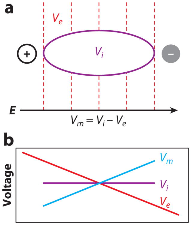
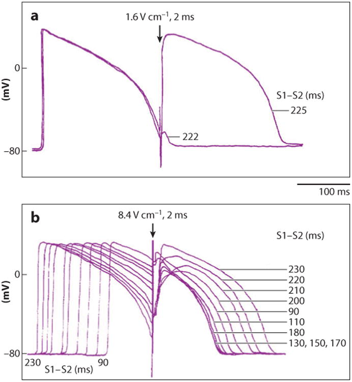
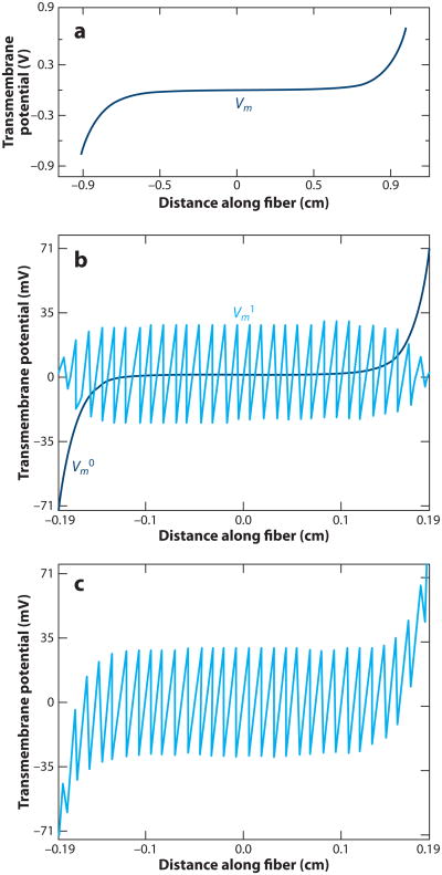
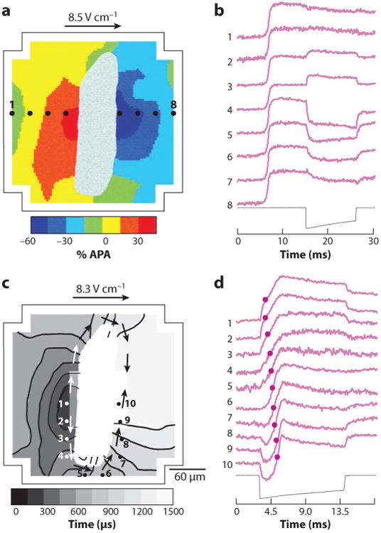
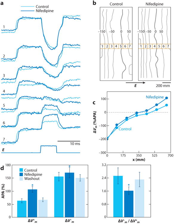
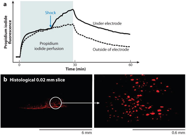
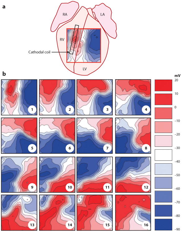
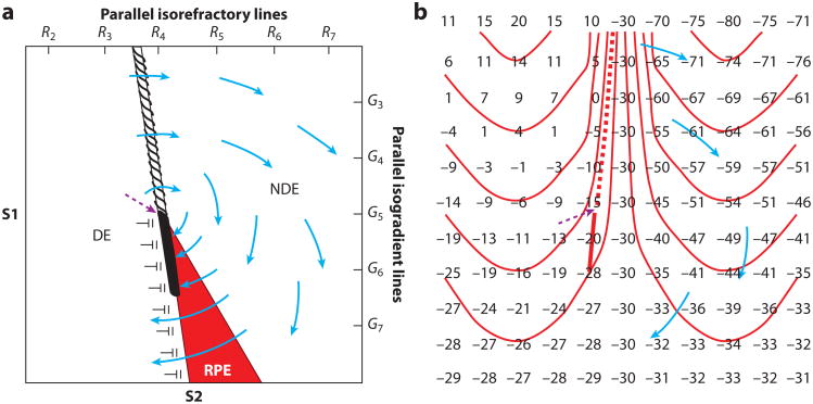
Electrical shock has been the one effective treatment for ventricular fibrillation for several decades. With the advancement of electrical and optical mapping techniques, histology, and computer modeling, the mechanisms responsible for defibrillation are now coming to light. In this review, we discuss recent work that demonstrates the various mechanisms responsible for defibrillation. On the cellular level, membrane depolarization and electroporation affect defibrillation outcome. Cell bundles and collagenous septae are secondary sources and cause virtual electrodes at sites far from shocking electrodes. On the whole-heart level, shock field gradient and critical points determine whether a shock is successful or whether reentry causes initiation and continuation of fibrillation.


Figures

Figure 1
Figure 1
Vm response in a single cell to an electric field. (a) Schematic of an elongated cell in an electric field. An electric field (E) creates a gradient of extracellular potential (Ve). Dashed lines indicate isopotential lines. Because of the relatively high impedance of the cell membrane and the short cell length, negligible amounts of current pass through the membrane, and the intracellular voltage (Vi) remains nearly constant throughout the cell. (b) Spatial profiles of Ve, Vi, and transmembrane potential (Vm) along the cell.
Figure 2
Figure 2
Varying strength and timing of shocks (S2) with respect to the previous electrical stimulus (S1) produce varying responses in recordings of transmembrane potential. (a) With a relatively weak shock field of 1.6 V cm−1, an all-or-nothing response is observed depending on the S1–S2 interval. With an S1–S2 interval of 222 ms, almost no response occurs. With an S1–S2 interval only 3 ms longer, 225 ms, a new action potential occurs. (b) A strong shock field of 8.4 V cm−1 during the plateau of an action potential produces a graded response that varies with the state of the cardiac cell when the shock was delivered. The S1–S2 interval was varied from 90 to 230 ms. The tracings are time aligned with the S2 shock (16).
Figure 3
Figure 3
Vm responses to uniform electric field predicted by the classical cable model and the sawtooth model. (a) The cable model predicts that Vm effects are limited to a group of cells in the immediate vicinity of the shocking electrodes. (b) The sawtooth model predicts a pattern of alternating positive and negative Vm changes (shown by Vm1) due to abrupt changes in intracellular resistivity across intercellular junctions. The cable model prediction is shown by Vm0. (c) The summed predicted ΔVm from the cable and sawtooth models (17).
Figure 4
Figure 4
Role of intercellular clefts in shock-induced ΔVm and tissue activation. (a) The shock-induced ΔVm surrounding a cleft in a myocyte monolayer follows the color scale on the bottom of the panel. White areas in the middle depict the intercellular cleft. The outline corresponds to the boundary of the photodiode array. APA, action potential amplitude. (b) Individual pixel recordings from sites 1–8 as shown in panel a with the shock waveform below. (c) Isochronal maps of activation spread initiated from secondary sources during application of shocks in diastole. The gray scale indicates the time of the isochronal lines. Arrows indicate the direction of activation spread. Activation times are determined from the time of earliest activation within the mapping region. (d) Individual pixel recordings from sites 1–10 from panel c. Activation times are shown with circles on the traces (31).
Figure 5
Figure 5
Shock-induced ΔVm in cell strands. (a) Schematic drawing of a cell strand and two photodiodes at opposite strand borders. (b) Recordings of ΔVm at strand border locations 1 and 2 during shocks of approximately 5 V cm−1 (green trace), 10 V cm−1 (blue trace), and 15 V cm−1 (purple trace). The shock field (E) for each shock is shown at the bottom. (c) The dependency of maximal positive and negative ΔVm at the opposite strand borders on the shock strength. Vertical dashed lines separate ranges with simple asymmetric ΔVm (II) from ranges with nonmonotonic ΔVm (III). No responses with symmetric ΔVm (I) are shown in this figure (107). APA, action potential amplitude.
Figure 6
Figure 6
Optical recording of ΔVm under a shocking electrode with different current densities. Arrows mark the beginning and end of the stimulus pulse. (a) Small timescale shows the nonmonotonic response of ΔVm to stimulus amplitude. (b) Large timescale shows elevation of the diastolic potential after the shock (38).
Figure 7
Figure 7
Computer simulation of a shock produces secondary sources in a model based on confocal microscopic images of ventricular rat tissue. (a) Progression of activation during a 10-ms shock. Transmembrane potentials of a single midvolume plane are shown according to the color scale at the top with cleavage plane discontinuities (black lines). Epi, epicardium; Endo, endocardium. (b) A three-dimensional view of secondary sources with transmembrane potentials greater than −60 mV at 2.5 ms into the shock (39).
Figure 8
Figure 8
Effects of shocks on intramural Vm in a porcine LV wedge preparation. (a) Optical recordings of Vm in control action potentials and during shock application. E, shock strength. The numbers correspond to the photodiodes indicated in panel b. (b) Isopotential maps of shock-induced ΔVm distribution measured at 9 ms after shock onset. The dashed lines indicate the epicardium on the left and the endocardium on the right (42). APA, action potential amplitude.
Figure 9
Figure 9
The role of Cai2+ current in asymmetric ΔVm during the action potential plateau. (a) Optical recordings of Vm from selected diodes and shock waveform taken in control and during nifedipine application in a strand with a width of 0.8 mm. The corresponding shock field strengths were 10.8 and 10.6 V cm−1. (b) Isopotential maps of ΔVm distribution 5 ms after the shock onset. Thick lines depict the zero isoline, which separates areas of depolarization and hyperpolarization. The seven numbered squares indicate the location of the diodes from which the recordings in panel a were made. (c) Spatial profiles of ΔVm across the strand. (d) Effect of nifedipine on optical ΔV+m, ΔVm, and the asymmetry ratio of ΔVm/ΔV+m in eight strands at a shock field strength of 9.3 ± 0.8 V cm−1 (49). APA, action potential amplitude.
Figure 10
Figure 10
Uptake of membrane-impermeable propidium iodide after a strong shock showing evidence of electroporation. (a) Propidium iodide fluorescence increased after a strong shock (1.6 A cm−2, 20 ms). (b) Fluorescence images made in the stimulation area show propidium iodide stained nuclei (38).
Figure 11
Figure 11
Transmembrane voltage after a failed defibrillation shock demonstrates the development of a virtual anode and cathode. (a) Approximate location of mapped area on the anterior surface of an optically mapped rabbit heart. RA, right atrium; LA, left atrium; RV, right ventricle; LV, left ventricle. (b) Each frame is 10 ms apart, starting from the first sample recorded after the end of the −100 V monophasic defibrillation shock. The virtual cathode (red) creates a wavefront that rapidly travels through the virtual anode (blue), which then reenters and reactivates the area originally occupied by the virtual cathode (62).
Figure 12
Figure 12
Two types of hypothesized critical points. (a) An idealized diagram is shown with a critical point (dashed purple arrow) formed at the intersection of a critical shock ∇V of G5 and a critical tissue refractoriness of R4. S1 pacing is performed from the left to cause a dispersion of refractoriness at the time of the S2 shock with R2 representing less and R7 more refractoriness. The S2 shock is given during the vulnerable period from the bottom of the region with large gradient G7 at the bottom and small gradient G3 at the top. The area on the left is sufficiently recovered so that it is directly excited (DE) by the gradient field. The area in the red region, although exposed to a higher gradient, is more refractory and undergoes refractory period extension (RPE), such that unidirectional block occurs from DE to RPE and activation in the DE tissue cannot propagate through this region. The region on the right is too refractory to be affected even with a large gradient and is not directly excited (NDE). Thus, propagation conducts unidirectionally from the DE to the NDE region at the top, encircling the critical point in a clockwise direction and reentering the DE region to create a reentrant circuit. (b) An idealized diagram is shown of a critical point (dashed purple arrow) caused by adjacent regions of depolarized and hyperpolarized transmembrane potential changes caused by the shock. Numbers represent transmembrane potentials at the end of the shock with isolines spaced every 10 mV beginning at −45 mV. The depolarized region (upper left) and the hyperpolarized region (upper right) are separated by a zone with a large gradient of membrane polarization, as indicated by the closely spaced isolines. The depolarized tissue in this zone is able to activate the adjacent hyperpolarized tissue to launch an activation front (dashed line) that propagates through the hyperpolarized region (blue arrows). Below, where the gradient in transmembrane potential is smaller, propagation cannot occur. A critical point is formed at the intersection of the frame and block lines where one end of the propagating activation front terminates in both panels. In both panels, the solid line represents the site of conduction block, and the dashed line indicates the location of the region from which an activation front is launched after the shock (108).
Figure 13
Figure 13
The spatial pattern of polarization at the end of the shock produced by a monophasic shock (+100 V, seventh ms of an 8-ms shock), optimal biphasic shock with more charge in the first than in the second phase (+100/−50 V, fifteenth ms of a 16-ms shock), and nonoptimal biphasic shock with less charge in the first than in the second phase (+100/−200 V, fifteenth ms of a 16-ms shock). The shocking electrodes were in the RV and above the right atrium, labeled ICD lead. The area from which the optical recordings were made is shown by the red box on the rabbit heart diagram. Values of polarization are shown relative to the preshock transmembrane voltage, with various gray levels assigned to positive and negative polarization, and white to areas of no polarization. RA, right atrium; LA, left atrium; RV, right ventricle; LV, left ventricle; BE, bipolar electrode (109).
Figure 14
Figure 14
Example of postshock cycles after a failed shock of a strength near the DFT delivered from electrodes in the RV apex and the superior vena cava. Recordings were made simultaneously from 504 electrodes distributed globally over the ventricular epicardium of a pig. Electrode sites are indicated in gray on a polar projection with the atrioventricular groove at the periphery and the LV apex in the center. Anterior is at the bottom of the projection, and the LV is to the right. Each panel shows in black the electrode sites at which an activation occurred at any time during a 10-ms interval. Numbers above the panels indicate the start of each 10-ms interval relative to the shock onset. Red arrows indicate the site of earliest recorded activation from each cycle. The first cycle appeared on the epicardium 64 ms after the shock at the anteroapical left ventricle. The second cycle (154 ms) arose on the epicardium in the same region as the first cycle and also propagated away in a focal pattern. The third (235-ms) and fourth (315-ms) cycles arose before the activation front from the previous cycle disappeared (78).

Similar articles

Cited by

References

    1. Hoffa M, Ludwig C. Einige neue Versuche über Herzebewegung. Z Ration Med. 1850;9:107–44.
    1. Prevost JL, Battelli F. Sur quelques effets des décharges électriques sur le coeur des Mammifères. C R Acad Sci. 1899;129:1267–68.
    1. Beck CS, Pritchard WH, Feil HS. Ventricular fibrillation of long duration abolished by electric shock. JAMA. 1947;135:985–86. - PubMed
    1. Zoll PM, Linenthal AJ, Gibson W, Paul MH, Norman LR. Termination of ventricular fibrillation in man by externally applied electric countershock. N Engl J Med. 1956;254:727–32. - PubMed
    1. Zipes DP, Fischer J, King RM, Nicoll A, Jolly WW. Termination of ventricular fibrillation in dogs by depolarizing a critical amount of myocardium. Am J Cardiol. 1975;36:37–44. - PubMed

Publication types

LinkOut - more resources