Analyzing Neuronal Networks Using Discrete-Time Dynamics

Abstract

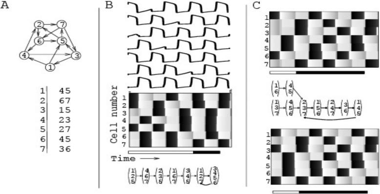
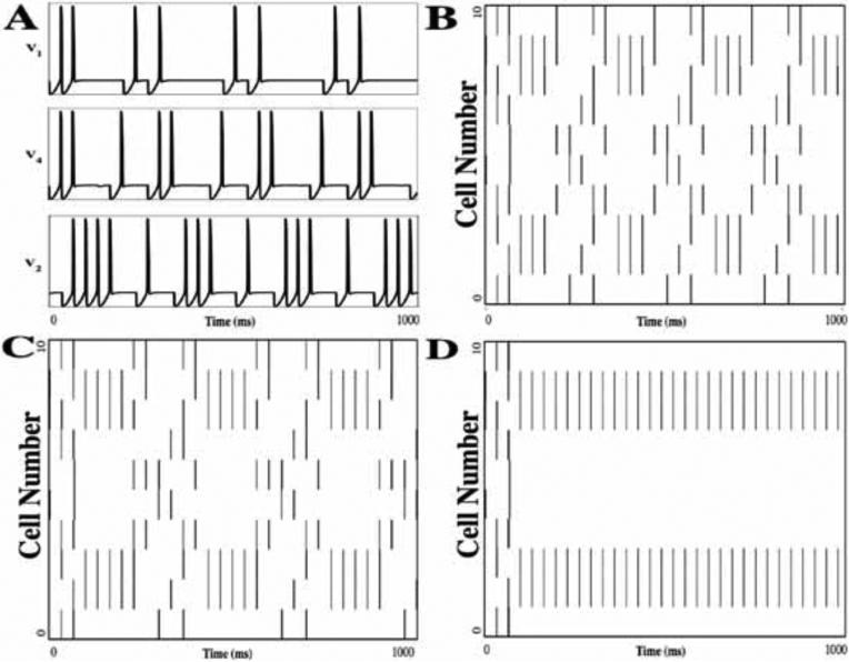
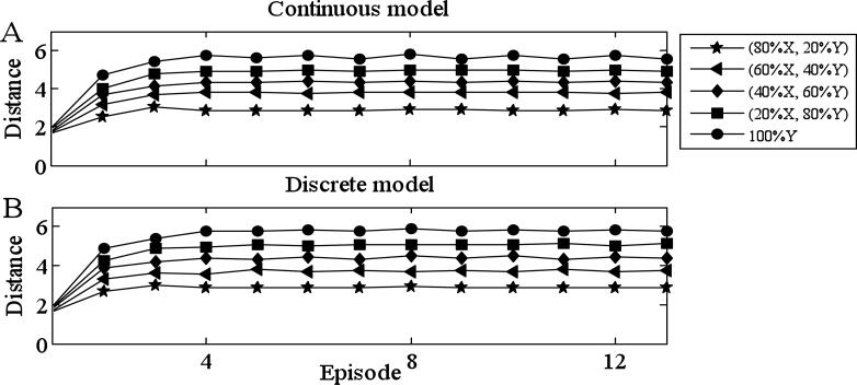
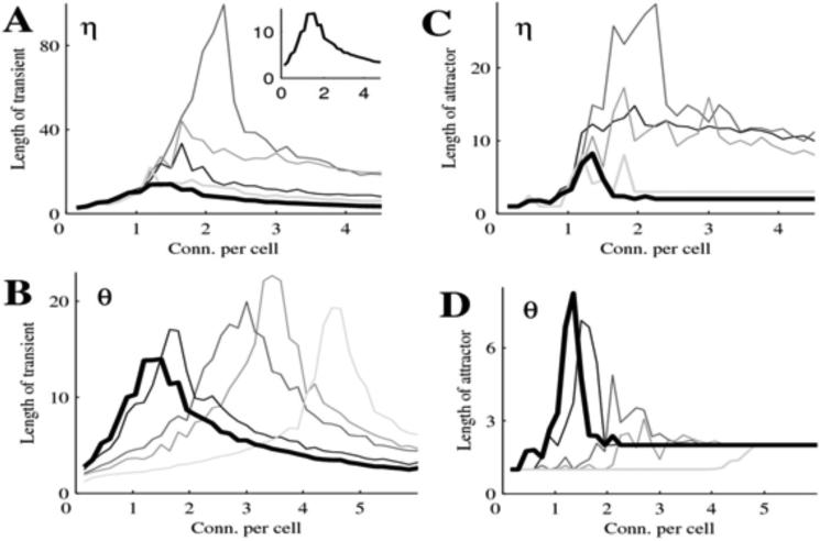
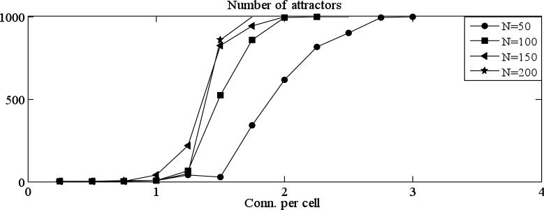
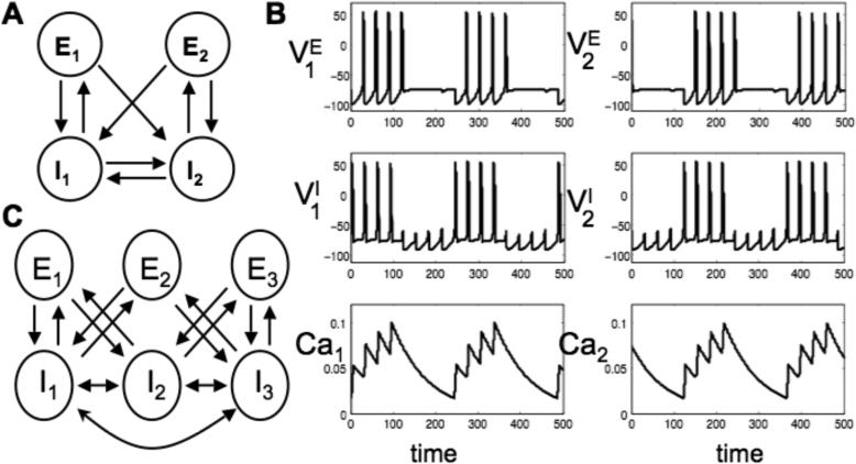
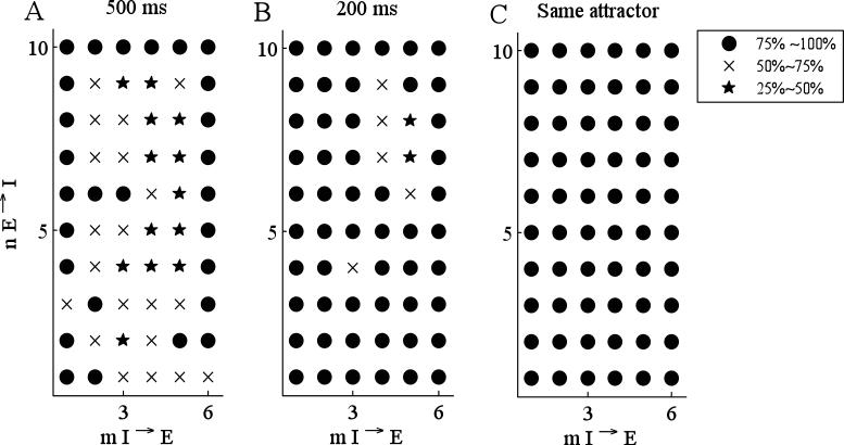
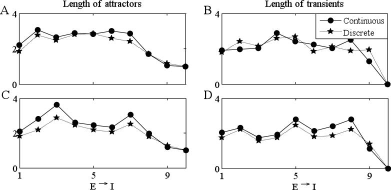
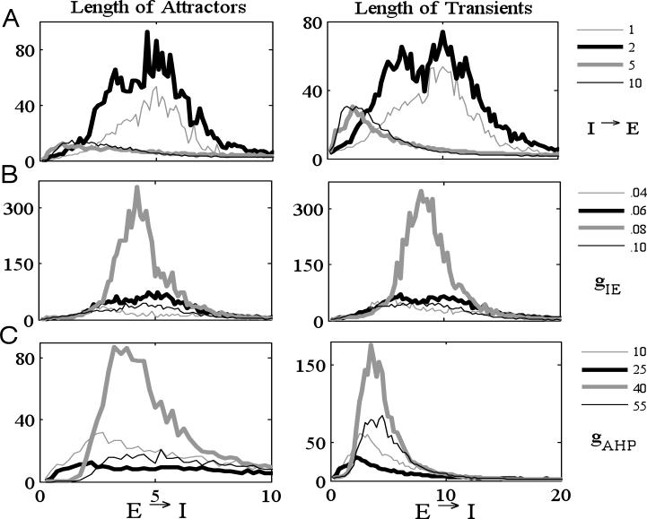
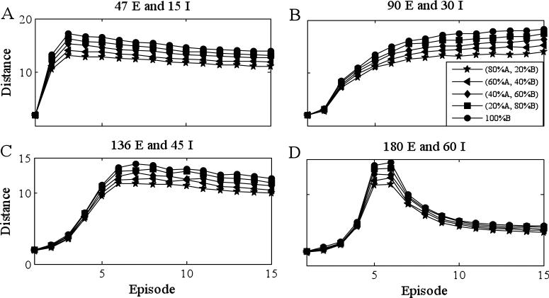
We develop mathematical techniques for analyzing detailed Hodgkin-Huxley like models for excitatory-inhibitory neuronal networks. Our strategy for studying a given network is to first reduce it to a discrete-time dynamical system. The discrete model is considerably easier to analyze, both mathematically and computationally, and parameters in the discrete model correspond directly to parameters in the original system of differential equations. While these networks arise in many important applications, a primary focus of this paper is to better understand mechanisms that underlie temporally dynamic responses in early processing of olfactory sensory information. The models presented here exhibit several properties that have been described for olfactory codes in an insect's Antennal Lobe. These include transient patterns of synchronization and decorrelation of sensory inputs. By reducing the model to a discrete system, we are able to systematically study how properties of the dynamics, including the complex structure of the transients and attractors, depend on factors related to connectivity and the intrinsic and synaptic properties of cells within the network.

Figure 1

An example of Model I. (A) The network consists of 7 cells with connections indicated by arrows. The connectivity is summarized in a table (bottom), in which the left column shows the indices of all cells, and the remaining columns show the indices of all cells that receive connections from the cell on the left. B) An example of network activity. The top panel shows the time courses of voltage in all 7 cells over 8 epochs of activity. Grey scale in the checkerboard panels corresponds to the magnitude of voltage, with black areas indicating spikes. After a transient (white part of the time bar under the checkerboard) the response converges to a repeating pattern (black part of the time bar). The bottom panel shows the orbit of the discrete dynamical system corresponding to this example. (C) Solutions of the same network, but with different initial conditions. These solutions have different transients (white parts of the time bars), but they converge to the same attractor (which, in turn, is different from the one in B).

Figure 2

An example of Model II dynamics. The network consists of 10 E-cells and 6 I-cells. Each E-cell receives input from 3 I-cells, chosen at random, and each I-cell receives input from 2 E-cells chosen at random, as well as all other I-cells. (A) The time course of voltage for three of the E-cells. A cell may fire for several subsequent episodes and then remain silent for several episodes. Two E-cells may fire synchronously during some episodes but not during others. (B) The entire E-cell network activity over 1000 ms. Each row corresponds to the activity of one of the E-cells; a vertical line indicates a spike. (C,D) Solutions of the same network as in panels A, B with different values of k_Ca (the rate of decay of calcium in the I-cells). In B, C and D, k_Ca = 2, 3.8 and 7, respectively. Values of other parameters are listed in Tables 1 and 2 except g_IE =.025, g_II =1.

Figure 3

Discrimination of odors. A network of 10 E- and 6 I-cells is presented with mixtures of two pure odors, X and Y. The pure odors activate disjoint subsets of 5 E-cells. For each fixed ratio of the two pure odors, 200 mixtures are randomly generated, as described in the text. The figure displays the distance (defined in the text) between the averaged firing pattern corresponding to the mixture and one of the pure odors (odor X) during each successive episode. The baseline is 100% odor X, different curves correspond to different ratios of X to Y: 80:20, 60:40, 40:60, 20:80 and 0:100. Values of other parameters are listed in Tables 1 and 2. (A) Full continuous model; (B) discrete counterpart (see section 5B).

Figure 4

Properties of transients and attractors in a 150-cells Model I network. Each point is averaged over 8 matrices of connectivity, and 1000 initial conditions for each matrix. (A,B) Properties of transients. (C,D) properties of attractors. Thick black curve (inset in A drawn to different scale) is the basic case when the threshold θ =0 and the refractory period η = 0. In the top row (A,C) different shades correspond to changes in the fraction of the cells with refractory period 2 (η). In the second row (B,D) different shades correspond to changing the fraction of the cells with threshold 2 (η). For each row changing of shade of thin lines from black to light grey corresponds, respectively, to η or η equaling 0.2, 0.5, 0.7, 1.

Figure 5

There are a huge number of attractors for sufficiently high connection probability. We computed the number of distinct attractors reached by solutions starting with a sample of 1000 random initial activation patterns. Note that for higher values of connectivity, each trajectory has its own attractor (the graphs reach 1000).

Figure 6

Two examples of Model II. (A) A model with two E- and two I-cells. (B) Activity of the model from A: voltage of the E-cells (top), voltage of the I-cells (middle) and calcium in the I-cells (bottom). E-I pairs take turns firing four action potentials. Activity in a pair stops when the calcium level in the I-cell becomes too large. (C) A network example with three E- and three I-cells. Properties of this network are discussed in the text.

Figure 7

Comparison between the continuous and the discrete models in a network of 10 E- and 6 I-cells. For each grid point at position (m,n), 20 networks are randomly chosen in which every I-cell receives connections from n E-cells and every E-cell receives connections from m I-cells. For each such network, 5 different initial conditions are chosen at random. The marker type corresponds to the percentage of simulations in which the continuous and the discrete models had the same firing patterns for A) 500 ms and B) 200 ms. In C), the marker type corresponds to the percentage of simulations in which the continuous and the discrete model reach the same attractor, regardless of the transient. Values of parameters are listed in Tables 1 and 2.

Figure 8

The discrete model predicts the lengths of attractors and transients. For each simulation used for Figure 7, we computed the lengths of attractors and transients and then averaged over all simulations corresponding to a fixed number of connections. (A) Attractors and transients for the same simulations as in column 4 in Figure 7. In (B), g_AHP is changed from 25 to 15 and k_Ca is changed from 20 to 35. Values of other parameters are listed in Tables 1 and 2.

Figure 9

Numerical simulations of the discrete model (100 E-cells and 40 I-cells). At each number of incoming connections, we considered 100 different random networks with 20 different initial conditions and then took the average length of attractor and transient. Each curve is plotted against the average number of E → I connections per cell. (A) Dependence of the lengths of attractors (left) and transients (right) on number of connections. Each curve represents a fixed number of I → E connections. (B,C) Dependence of lengths of attractors and transients on parameters g_IE (B) and g_AHP (C). Here we fixed the number of I → E connections (2 I → E in (B) and 5 I → E in (C)). Same parameter values as in Tables 1 and 2.

Figure 10

Discrimination of odors for the discrete model, larger network (300 E-cells, 100 I-cells). Each pure odor corresponds to the activation of 30 E-cells and the two odors activated non-overlapping sets of E-cells. Different panels correspond to different number of connections in the network. The figure displays the distance (defined in the text) between the averaged firing pattern corresponding to the mixture and one of the pure odors (odor X). For each connection probability, we used 1000 different networks and initial conditions and then took the average distance. The baseline is 100% odor X, different curves correspond to ratios of odors X to Y: 80:20, 60:40, 40:60, 20:80 and 0:100. Values of other parameters are listed in Tables 1 and 2 except k_Ca =15 and g_AHP =55.

References

1. Llinas RR. The intrinsic electrophysiological properties of mammalian neurons: Insights into central nervous system function. Science. 1988;242:1654–1664. - PubMed
1. Jacklet JW. Neuronal and Cellular Oscillators. Marcel Dekker Inc; New York: 1989.
1. Steriade M, Jones EG, Llinas RR. Thalamic Oscillations and Signaling. Wiley; New York: 1990.
1. Steriade M, Jones E, McCormick D, editors. Thalamus. II. Elsevier; Amsterdam: 1997.
1. Traub RD, Miles R. Neuronal Networks of the Hippocampus. Cambridge University Press; New York: 1991.
LinkOut - more resources