The role of V1 surround suppression in MT motion integration

Abstract

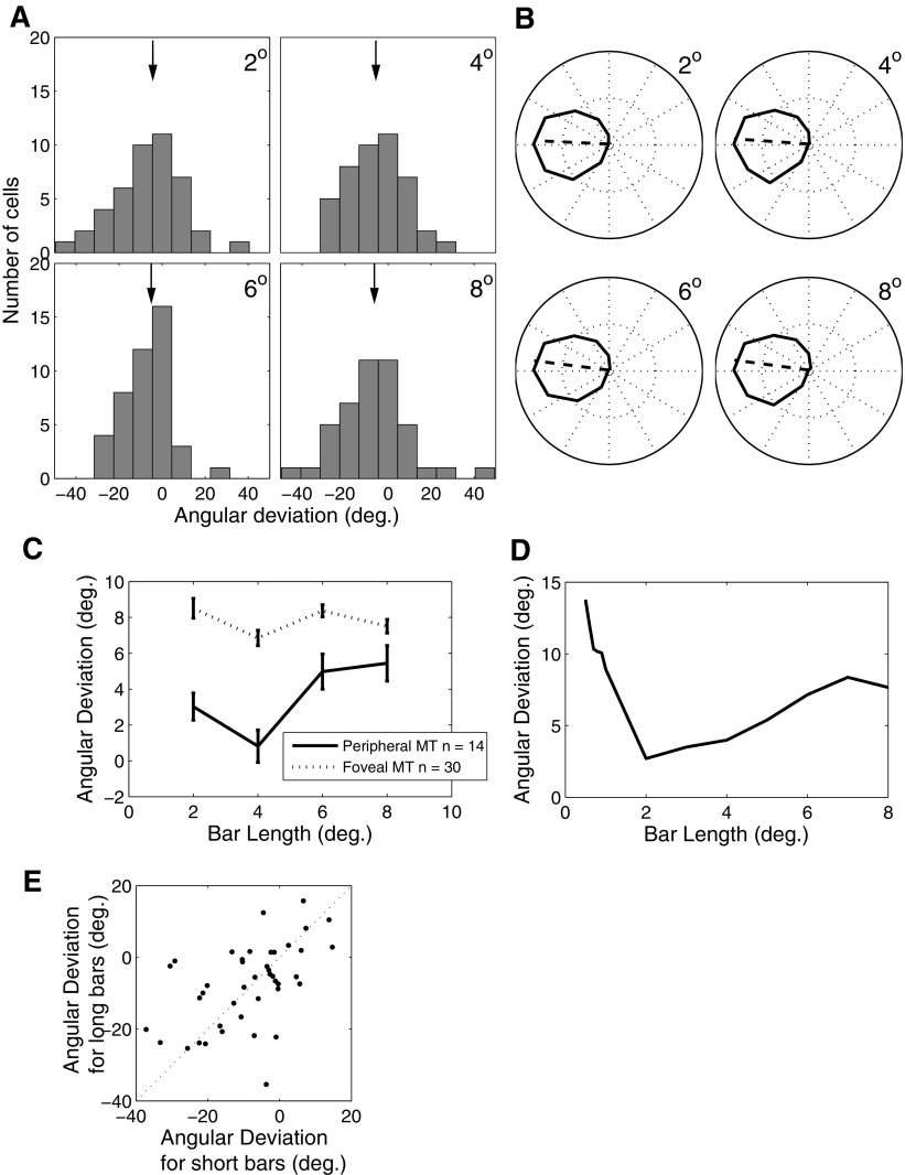
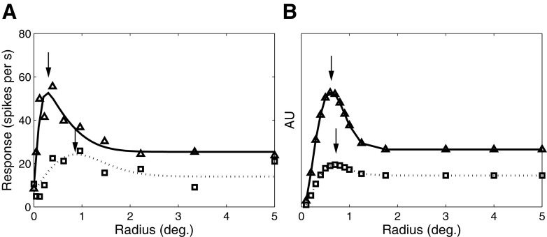
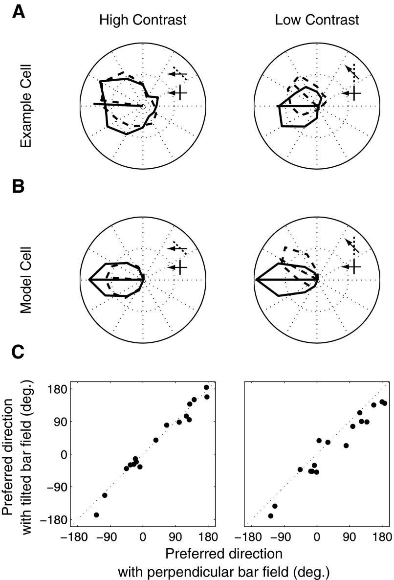
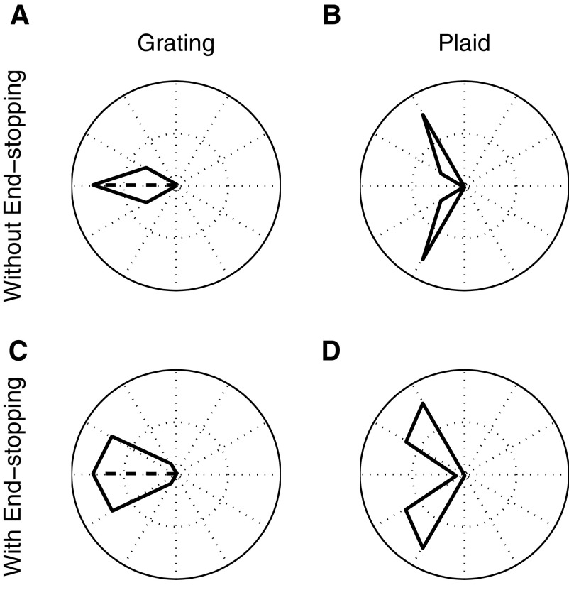
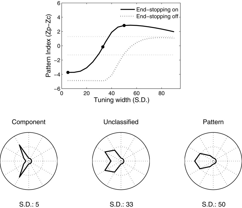
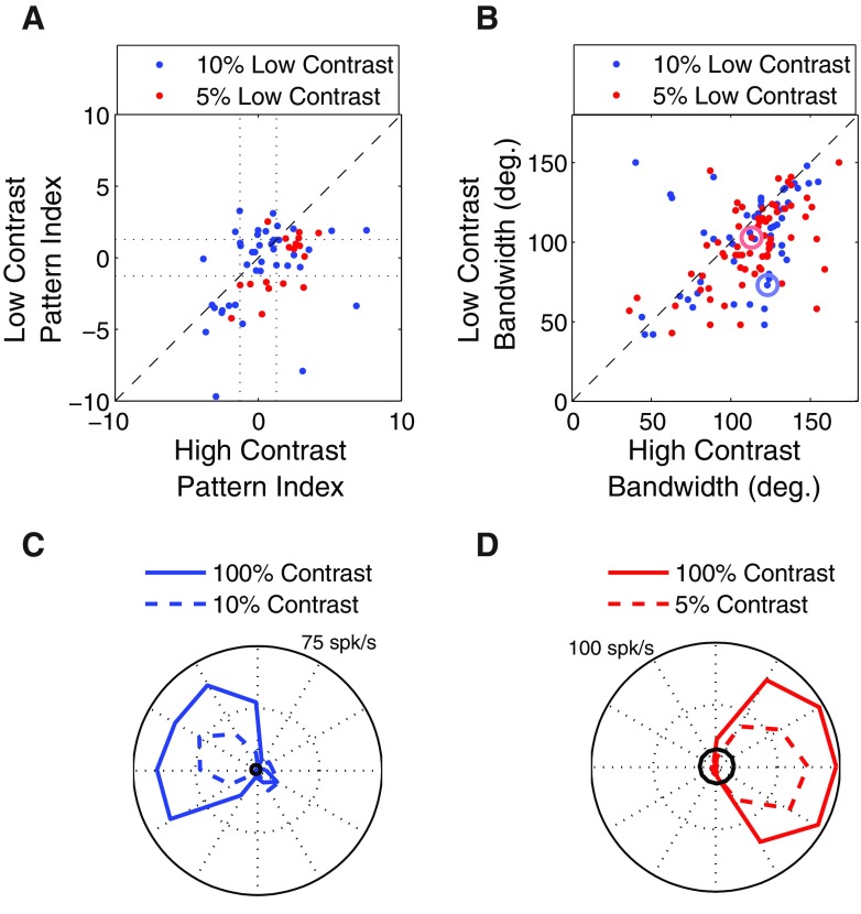
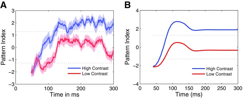
Neurons in the primate extrastriate cortex are highly selective for complex stimulus features such as faces, objects, and motion patterns. One explanation for this selectivity is that neurons in these areas carry out sophisticated computations on the outputs of lower-level areas such as primary visual cortex (V1), where neuronal selectivity is often modeled in terms of linear spatiotemporal filters. However, it has long been known that such simple V1 models are incomplete because they fail to capture important nonlinearities that can substantially alter neuronal selectivity for specific stimulus features. Thus a key step in understanding the function of higher cortical areas is the development of realistic models of their V1 inputs. We have addressed this issue by constructing a computational model of the V1 neurons that provide the strongest input to extrastriate cortical middle temporal (MT) area. We find that a modest elaboration to the standard model of V1 direction selectivity generates model neurons with strong end-stopping, a property that is also found in the V1 layers that provide input to MT. With this computational feature in place, the seemingly complex properties of MT neurons can be simulated by assuming that they perform a simple nonlinear summation of their inputs. The resulting model, which has a very small number of free parameters, can simulate many of the diverse properties of MT neurons. In particular, we simulate the invariance of MT tuning curves to the orientation and length of tilted bar stimuli, as well as the accompanying temporal dynamics. We also show how this property relates to the continuum from component to pattern selectivity observed when MT neurons are tested with plaids. Finally, we confirm several key predictions of the model by recording from MT neurons in the alert macaque monkey. Overall our results demonstrate that many of the seemingly complex computations carried out by high-level cortical neurons can in principle be understood by examining the properties of their inputs.

Fig. 1.

Stimuli used in the simulations. A: tilted bar stimulus. The orientation of the bar is rotated 45° counterclockwise with respect to its direction of motion. The direction of motion measured at the endpoints contains 2-dimensional features corresponding to the veridical motion direction. The edge of the bar contains only one-dimensional features that correspond to the direction of motion perpendicular to stimulus orientation. The ambiguity of these signals results from the aperture problem. B: plaid stimulus. The plaid stimulus is composed of 2 gratings drifting in different directions of motion (top). When the gratings are superimposed (bottom) the perceived direction of the resulting pattern corresponds to the motion of neither component.

Fig. 2.

Model. A: motion energy model (adapted from Adelson and Bergen 1985). The stimulus is processed by 2 spatial filters and the resulting outputs are convolved with several temporal filters, recombined, squared, summed, and passed through a square root operation prior to the computation of an opponent stage. See methods for details. The end-stopped stage is added at the initial stage (dotted box, top right). B: middle temporal (MT) model. The MT cell receives input from a population of primary visual cortex (V1) cells with spatially shifted receptive fields. The output is determined by summing over these inputs with SoftMax weighting.

Fig. 3.

Model MT responses without V1 end-stopping. The tuning curve at the center shows the response of a model MT cell preferring leftward motion to a tilted bar moving in various directions, with an orientation that is tilted by 45° with respect to the direction of motion (bar/arrow icons). The angular deviation from the preferred direction of motion of the MT cell is 33.4°. Each peripheral panel shows the population responses, wherein each pixel corresponds to the activity of a single model V1 cell that prefers leftward motion.

Fig. 4.

MT responses with end-stopping. Conventions are the same as those in Fig. 3. The peripheral panels show that the endpoints evoke stronger responses than the edges of the bar and the central panel shows the tuning curve, which has a preferred direction that now deviates by only 3.5° from leftward.

Fig. 5.

Angular deviation as a function of the surround suppression strength. Angular deviation is the rotation of the tuning curve introduced by tilting the bar stimulus by 45°. The figure shows this value for the model with surrounds consisting of 3 side-stopped units (blue line), 7 side-stopped units (green line), 3 end-stopped units (red line), 7 end-stopped units (cyan line), homogeneous inhibition (magenta line), and end-stopped units with multiple preferred orientations (brown line). The surround suppression strength was manipulated by varying the parameter k that controls the strength of inhibition (see methods). The configurations with end-stopping units lead to small errors.

Fig. 6.

Angular deviation as a function of bar length. A: distribution of angular deviations in a population of 44 MT cells for tilted bars of different lengths. The black arrows in each panel indicate the median angular deviation values (4.8, 6.6, 5.8, and 7.3° for 2, 4, 6, and 8° bar lengths, respectively). B: tuning curves from the model for different bar lengths. The correspondent angular deviation values are 2.7, 4.0, 7.2, and 7.7°. C: angular deviation as a function of bar length for central (dotted) and peripheral (solid) cells. Cells were considered peripheral if they had an eccentricity of >10°. D: same as C for the model. E: cell-by-cell correlation of angular deviation values for long (8°) vs. short (2°) bars.

Fig. 7.

Effect of contrast on spatial summation in V1. A: size tuning for a complex cell from layer 4B for high (triangles) and low (squares) contrasts (adapted from Sceniak et al. 1999). B: model end-stopped responses as a function of stimulus size. The solid and dotted traces correspond to the responses elicited by high- and low-contrast drifting gratings. For both the model and real V1 cells, the optimal size (black arrows) increases and the suppression strength decreases as contrast decreases.

Fig. 8.

Effect of contrast on angular deviation. A: an example MT cell. The solid and dotted traces correspond to the tuning curves for bar field stimuli with no tilt and a 45° tilt at high (left) and low (right) contrasts. The bar/arrow icons show the configuration of a stimulus moving at the cell's preferred direction for the 2 tilt conditions. The arrows and bars illustrate the configurations that evoked the strongest responses. B: responses of the model MT cell under the same conditions. C: preferred directions for the tilted bar at high (left) and low (right) contrasts for 17 MT cells. At low contrast, the points lie below unity line, indicating an increase in angular deviation.

Fig. 9.

A: the temporal dynamics of angular deviation for different values of the delay parameter d (blue: d = 0; green: d = 8 ms, red: d = 16 ms, cyan: d = 24 ms; and magenta: d = 32 ms). B: mean responses of 17 MT cells as a function of time for high-contrast (blue) and low-contrast (red) bar stimuli. C: model response to the high- (blue) and low-contrast (red) bar stimuli.

Fig. 10.

Tuning curves for grating (left) and plaid (right) stimuli. A and B: MT model responses to the grating and plaid stimuli with end-stopping turned off. The bilobed tuning curve for the plaid stimulus is consistent with component selectivity. C and D: same as A and B with end-stopping turned on. Again, the model is strongly component-selective.

Fig. 11.

Pattern index for varying integration bandwidths. The solid and dotted traces show the pattern index when end-stopping is turned on and off, respectively. As the bandwidth of integration increases, pattern selectivity increases gradually. However, the model does not achieve statistically significant pattern selectivity (top dashed horizontal line) without end-stopping. For narrow bandwidths the model is component-selective (bottom dashed horizontal line), irrespective of the presence or absence of end-stopping. The polar plots at the bottom of the figure correspond to the tuning curves for the model with bandwidths given by the solid dots in the top panel. These example model responses from left to right are characterized as component, unclassified, and pattern.

Fig. 12.

Effect of contrast on pattern index and tuning bandwidth. A: pattern index for 58 MT cells at high and low contrasts. The points lying below the unity line indicate a tendency to become more component-selective at low contrast. B: tuning bandwidth for 133 MT cells in response to a grating stimulus. The points lying below the unity line indicate a tendency to become more narrowly tuned at low contrast. The circled dots correspond to the example neurons in C and D. C: direction tuning curves at high (solid line) and low (dashed line) contrast for the example neuron indicated by the large blue circle in B. Black circle indicates 2SDs above the mean of the baseline firing rate. D: as in C, but for the neuron indicated by the large red circle in B.

Fig. 13.

A: the average plaid temporal dynamics of 23 MT pattern cells from Fig. 12A. The pattern index (see methods) was computed in 24 ms time bins. At high contrast (blue), the pattern index switches gradually from an early, component-selective response to a later pattern-selective response over a period of roughly 75 ms. The pattern index transition at low contrast occurs on a similar timescale, but fails to reach statistical significance. B: same as A for the model.

References

1. Adelson EH, Bergen JR. Spatiotemporal energy models for the perception of motion. J Opt Soc Am A 2: 284–299, 1985. - PubMed
1. Adelson EH, Movshon JA. Phenomenal coherence of moving visual patterns. Nature 300: 523–525, 1982. - PubMed
1. Albrecht DG. Visual cortex neurons in monkey and cat: effect of contrast on the spatial and temporal phase transfer functions. Vis Neurosci 12: 1191–1210, 1995. - PubMed
1. Albright TD. Direction and orientation selectivity of neurons in visual area MT of the macaque. J Neurophysiol 52: 1106–1130, 1984. - PubMed
1. Angelucci A, Levitt JB, Walton EJ, Hupe JM, Bullier J, Lund JS. Circuits for local and global signal integration in primary visual cortex. J Neurosci 22: 8633–8646, 2002. - PMC - PubMed
Publication types
LinkOut - more resources