Measuring phase-amplitude coupling between neuronal oscillations of different frequencies

Abstract

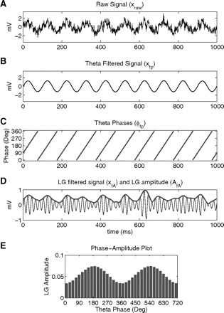
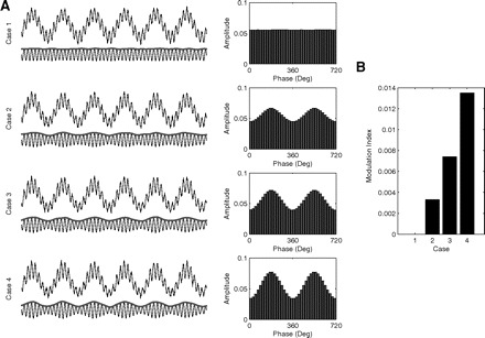
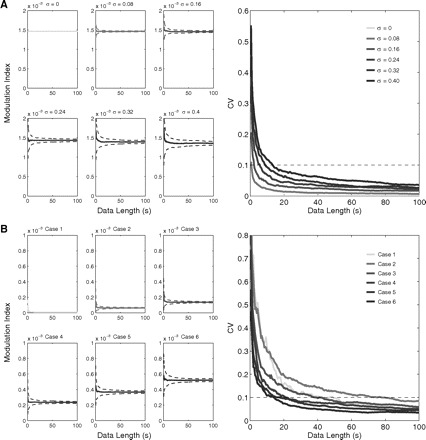
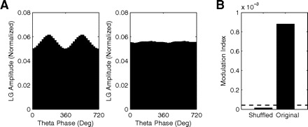
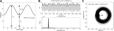
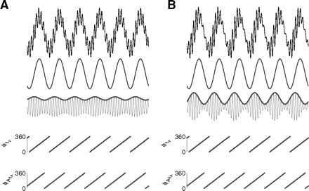
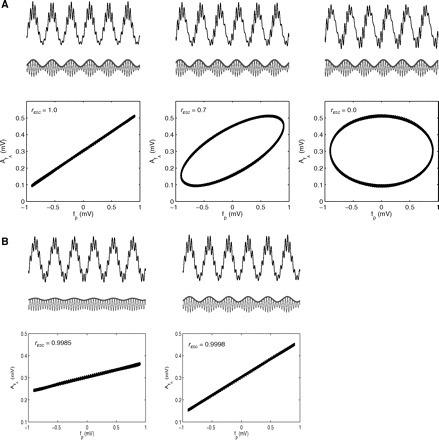
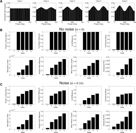
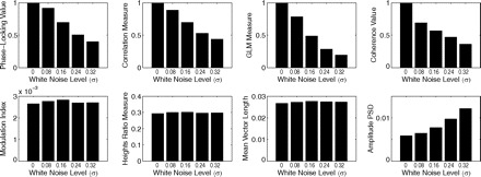
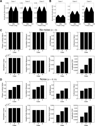
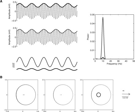
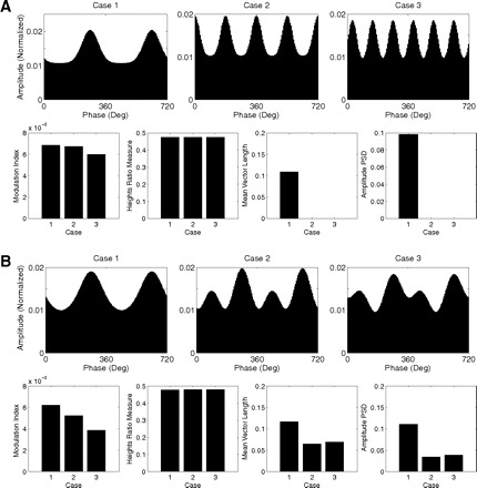
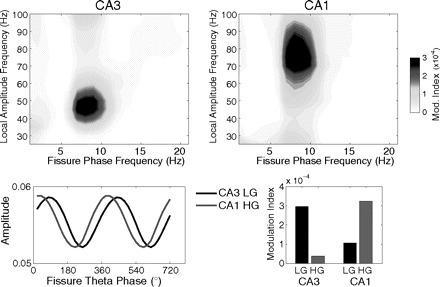
Neuronal oscillations of different frequencies can interact in several ways. There has been particular interest in the modulation of the amplitude of high-frequency oscillations by the phase of low-frequency oscillations, since recent evidence suggests a functional role for this type of cross-frequency coupling (CFC). Phase-amplitude coupling has been reported in continuous electrophysiological signals obtained from the brain at both local and macroscopic levels. In the present work, we present a new measure for assessing phase-amplitude CFC. This measure is defined as an adaptation of the Kullback-Leibler distance-a function that is used to infer the distance between two distributions-and calculates how much an empirical amplitude distribution-like function over phase bins deviates from the uniform distribution. We show that a CFC measure defined this way is well suited for assessing the intensity of phase-amplitude coupling. We also review seven other CFC measures; we show that, by some performance benchmarks, our measure is especially attractive for this task. We also discuss some technical aspects related to the measure, such as the length of the epochs used for these analyses and the utility of surrogate control analyses. Finally, we apply the measure and a related CFC tool to actual hippocampal recordings obtained from freely moving rats and show, for the first time, that the CA3 and CA1 regions present different CFC characteristics.

Fig. 1.

Steps in the computation of the phase-amplitude plot and modulation index (MI). The raw signal (A) is filtered at the phase (B) and amplitude (D, thin line) frequency ranges of interest. Next the phase (C) and the amplitude (D, thick line) time series are calculated from the filtered signals by using the Hilbert transform. A composite phase-amplitude time series (ϕ_fp, A_fA) is then constructed and used to obtain the mean amplitude distribution over phase bins (E; 2 cycles shown for clarity). The MI is obtained by measuring the divergence of the observed amplitude distribution from the uniform distribution. See text for further details. LG, low-gamma (30–60 Hz).

Fig. 2.

Modulation index performance in assessing phase-amplitude coupling. A, left: 4 cases differing in coupling strength are shown (top traces) along with their corresponding phase-amplitude plots (right panels). The thin and the thick traces plotted underneath show the LG filtered signal and its amplitude envelope, respectively. B: MI values for the 4 example cases shown in A.

Fig. 3.

Dependence of the MI on the data length. A: plots in the left show the mean MI value as a function of the data length for 6 cases of theta–LG coupling differing in noise intensity (σ² is the variance of the white noise process; see appendix). Dashed lines denote ±SD; 100 trials were simulated for each parameter set. Notice that the mean MI approaches a steady value and that the variance among trials gets reduced with longer data lengths. The corresponding coefficient of variation (CV) levels are shown in the right plot. B: CV levels (right plot) as a function of the data length for 6 cases of theta–LG coupling differing in coupling strength (left plots). Noise level was fixed at σ = 0.24.

Fig. 4.

Surrogate control analysis. A: theta–LG phase-amplitude plots obtained for the original (left) and a representative trial-shuffled [ϕ_fp(t), A_fA(t)] time series (right) derived from actual hippocampal data. B: mean MI for 200 trial-shuffled and the original phase-amplitude time series. Dashed line represents the significance threshold.

Fig. 5.

Principles underlying 3 phase-amplitude cross-frequency coupling (CFC) measures. A: the heights ratio measure can be straightforwardly defined in a phase-amplitude plot, as indicated. B: the power spectral density (PSD) of the instantaneous amplitude envelope can be used to assess phase-amplitude coupling. In this example, a theta–LG coupling measure can be defined by integrating the power values over the theta band. C: a phase-amplitude coupling measure can be defined as the length of the mean vector (arrow) of a time series defined in the complex plane by A_fAe^i∗ϕ_fp (black dots connected with line). Notice the existence of asymmetry around zero in this example, which characterizes the existence of phase-amplitude coupling in this analysis.

Fig. 6.

Assessing the phase-locking between the amplitude envelope A_fA and f_p. A, top panels: shown are a synthetic local field potential (LFP) example, along with the signal filtered at theta and gamma ranges bottom traces. The amplitude envelope (A_fA) of the gamma filtered signal is also shown (thick line). Bottom panels: phase time series of theta (top) and gamma amplitude (bottom). B: same as before but for a case with stronger phase-amplitude coupling (as judged by the amplitude envelope). Notice that the phase-time series of the amplitude envelope is identical to the previous case and thus the levels of phase-locking to the f_p rhythm are the same. Therefore CFC measures dependent on the level of phase-locking between A_fA and f_p are, in principle, potentially not able to track CFC intensity (for better clarity of the proof of principle, no noise was added to the synthetic signals shown in this figure).

Fig. 7.

Assessing the linear regression between the amplitude envelope A_fA and f_p. A, top panels: 3 cases of phase-amplitude coupling presenting the same intensity (as judged by the amplitude envelope) but different coupling phases (top trace: synthetic LFP; bottom traces: gamma filtered signal (thin line) and gamma amplitude envelope (thick line)). Bottom panels: scatterplots between f_p and A_fA, which show that the correlation coefficient (r_ESC) depends on the phase lag between A_fA and f_p. B: 2 cases differing in CFC strength. Notice that the correlation coefficient provides similar results, since it does not depend on the slope of the regression nor on its y-intercept. Therefore CFC measures dependent on the regression between A_fA and f_p do not, in principle, correlate well with its intensity (for better clarity of the proof of principle, no noise was added to the synthetic signals shown in this figure).

Fig. 8.

Performance comparison among 8 phase-amplitude coupling measures. A: 5 cases differing in coupling strength were analyzed. B: CFC measures values for the 5 cases shown in A in the absence of noise. Notice that the phase-locking index, the correlation measure, the general linear model (GLM) measure, and the coherence value are all able to detect phase-amplitude coupling, but do not distinguish well between different levels of coupling strength. C: similar to the above, but in the presence of noise. All measures are then able to track coupling intensity.

Fig. 9.

Influence of noise level on the coupling measures.

Fig. 10.

Influence of the absolute amplitude of the amplitude-modulated band on the coupling measures. A and B: 3 cases of identical coupling strength, but differing in the absolute amplitude of f_A are shown. Panels in A show the normalized amplitude (i.e., the distribution-like function P; see methods), whereas panels in B show the absolute mean amplitude level per phase bin for the same 3 cases. C: CFC measures values for the 3 cases depicted in A and B in the absence of noise. D: same as the above, but in the presence of noise.

Fig. 11.

Amplitude dependence of 2 CFC measures. A, left panels: shown are 2 gamma filtered signals (top thin traces) along with their amplitude envelopes (thick traces). Notice that both examples present a similar level of phase-amplitude coupling and that the y-scale is different between both panels; the amplitude of the gamma oscillation in the second example (gray) is fivefold higher than the first (black). The bottom panel shows both amplitude envelopes plotted in the same y-scale. Right: PSD of the amplitude envelopes (same color scheme), showing that the amplitude PSD measure is dependent on the absolute amplitude. B, left 2 panels: complex plane representation of the A_fAe^i∗ϕ_fp time series obtained from the examples in A, along with their mean vector length (same color convention). Notice the different x- and y-scales. When plotted in the same scale (3rd plot from left), the different gamma amplitudes become evident. The rightmost panel shows the mean vectors for both examples plotted in the same scale. The mean vector length measure is therefore dependent on the absolute amplitude of f_A.

Fig. 12.

Sensitivity of the coupling measures to the “width” of the amplitude modulation by phase. A: 2 example cases plotted simultaneously (black and gray curves) illustrating that the “modulation width” can vary for the same maximal and minimal heights. B: CFC measures values (bottom) for 5 cases varying in modulation width (top).

Fig. 13.

Sensitivity of the coupling measures to multimodal amplitude distributions. A and B: CFC measures values for 3 cases of symmetric (A) and asymmetric (B) multimodal amplitude distributions.

Fig. 14.

Characteristics of the gamma amplitude modulation by theta-phase differ between the CA1 and CA3 regions. Top panels: representative phase-amplitude comodulograms computed for CA3 (left) and CA1 (right) LFPs recorded simultaneously (at s. pyramidale) during context exploration. A common electrode located at the hippocampal fissure was used as the phase reference. Bottom panels: mean amplitude (normalized) per theta phase of LG in CA3 (black) and HG in CA1 (gray) for the same electrodes (left). The associated MI values are also shown (right).

References

1. Axmacher N, Henseler MM, Jensen O, Weinreich I, Elger CE, Fell J. Cross-frequency coupling supports multi-item working memory in the human hippocampus.Proc Natl Acad Sci USA 107: 3228–3233, 2010 - PMC - PubMed
1. Bragin A, Jando G, Nadasdy Z, Hetke J, Wise K, Buzsáki G. Gamma (40–100 Hz) oscillation in the hippocampus of the behaving rat.J Neurosci 15: 47–60, 1995 - PMC - PubMed
1. Buzsáki G, Buhl DL, Harris KD, Csicsvari J, Czeh B, Morozov A. Hippocampal network patterns of activity in the mouse.Neuroscience 116: 201–211, 2003 - PubMed
1. Canolty RT, Edwards E, Dalal SS, Soltani M, Nagarajan SS, Kirsch HE, Berger MS, Barbaro NM, Knight RT. High gamma power is phase-locked to theta oscillations in human neocortex.Science 313: 1626–1628, 2006 - PMC - PubMed
1. Cohen MX. Assessing transient cross-frequency coupling in EEG data.J Neurosci Methods 168: 494–499, 2008 - PubMed
Publication types
LinkOut - more resources