Dynamics of bacterial swarming

Abstract

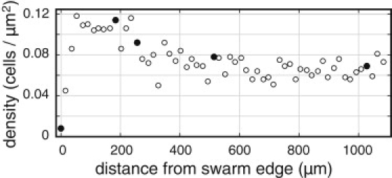
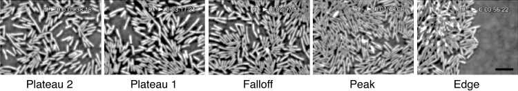
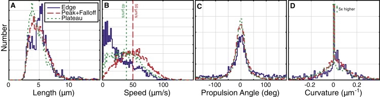
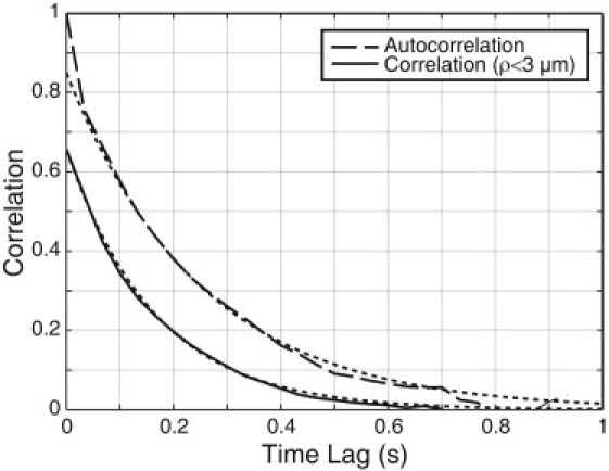
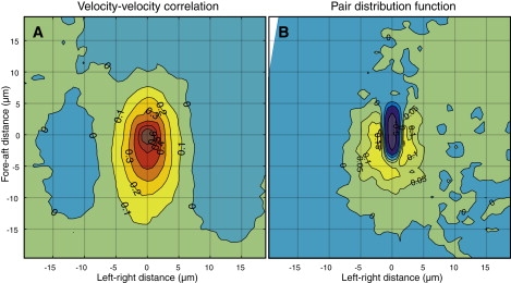
When vegetative bacteria that can swim are grown in a rich medium on an agar surface, they become multinucleate, elongate, synthesize large numbers of flagella, produce wetting agents, and move across the surface in coordinated packs: they swarm. We examined the motion of swarming Escherichia coli, comparing the motion of individual cells to their motion during swimming. Swarming cells' speeds are comparable to bulk swimming speeds, but very broadly distributed. Their speeds and orientations are correlated over a short distance (several cell lengths), but this correlation is not isotropic. We observe the swirling that is conspicuous in many swarming systems, probably due to increasingly long-lived correlations among cells that associate into groups. The normal run-tumble behavior seen in swimming chemotaxis is largely suppressed, instead, cells are continually reoriented by random jostling by their neighbors, randomizing their directions in a few tenths of a second. At the edge of the swarm, cells often pause, then swim back toward the center of the swarm or along its edge. Local alignment among cells, a necessary condition of many flocking theories, is accomplished by cell body collisions and/or short-range hydrodynamic interactions.

Figure 1

Swarm density profile. Cell-density profile for the first swarm from Table 1 (open symbols). Cells were counted in each video frame collected at 5-s intervals for a total of 300 s. Solid symbols denote the regions selected for further study, in the order (left to right) edge, peak, falloff, plateau 1, and plateau 2.

Figure 2

Snapshots of an advancing swarm. Images of cells in regions corresponding to the solid symbols in Fig. 1. The field of view is (42 μm) × (57 μm). Scale bar = 10 μm. The cells are shown in the order and orientation appropriate for swarms moving from left to right.

Figure 3

Population distributions. Distributions of body length, speed, propulsion angle, and curvature, each grouped by the location of the cells in the swarm: at the edge (solid blue), in the peak and falloff regions (dashed red), and in the two lower-density plateau regions (dotted green). Distributions of each type are normalized to the same area. Vertical lines on the speed distribution indicate mean values. The peaks at zero in the curvature distributions are truncated: they are 5× larger than pictured and contain ∼50% of the total distribution. Note that ∼40% of all measured trajectories were omitted from the curvature distribution because they failed to fit to an arc of a circle. See Methods for details.

Figure 4

Temporal correlations. The velocity-velocity temporal correlation function (solid line, lower) represents the time over which the velocity of cells in a small (3 μm square) spatial region of the swarm becomes randomized. A 0.17 s exponential decay (dotted line) is included for reference. The correlation at t = 0 is <1 because the 3 μm spatial binning averages over several cells that are initially imperfectly aligned. Because the particular cells located within the 3 μm bins change over time, the temporal correlation function is a property of the swarm rather than of its individual cells. The velocity-velocity temporal autocorrelation function (dashed line, upper) represents the time over which an individual cell's velocity becomes randomized. A 0.25-s exponential decay (dotted line) is included for reference. Due to the finite size of our video frame, we are susceptible to sampling bias for times beyond a few tenths of a second (because cells that consistently move in the same direction tend to swim out of our field of view), so we are not confident in the long-time tail of the autocorrelation function. See Methods for formal definitions of correlation and autocorrelation functions.

Figure 5

Spatial correlations. (A) The velocity-velocity spatial correlation function represents the degree of directional alignment between velocities of different cells as a function of distance. (B) The pair distribution function represents the probability of finding two cells a certain distance apart. The dark blue region of low probability around the origin is due to mutual exclusion by the 1 μm × 5 μm cell bodies. A second cell is ∼10% more likely than average to be located near the side and back of another cell. Outside of the exclusion zone, the error on the velocity-velocity correlation (A) is ∼0.015 and the error on the pair distribution function (B) varies from 0.03 to 0.02 with increasing distance from the origin. See Methods for definitions of these functions and of the coordinate system.

References

-
- Berg H.C., Anderson R.A. Bacteria swim by rotating their flagellar filaments. Nature. 1973;245:380–382. - PubMed
- Berg H.C. Springer; New York: 2004. E. coli in Motion.
- Baker M.A.B., Berry R.M. An introduction to the physics of the bacterial flagellar motor: a nanoscale rotary electric motor. Contemp. Phys. 2009;50:617–632.
- Sowa Y., Berry R.M. Bacterial flagellar motor. Q. Rev. Biophys. 2008;41:103–132. - PubMed
- Terashima H., Kojima S., Homma M. Flagellar motility in bacteria structure and function of flagellar motor. Int. Rev. Cell Mol. Biol. 2008;270:39–85. - PubMed
Publication types
MeSH terms
Substances
Grants and funding
LinkOut - more resources
Full Text Sources
Other Literature Sources
Molecular Biology Databases