From moonlight to movement and synchronized randomness: Fourier and wavelet analyses of animal location time series data

Abstract

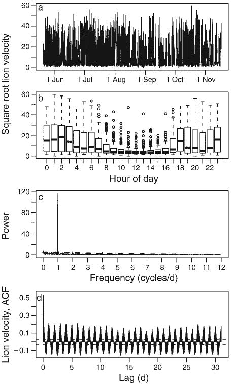
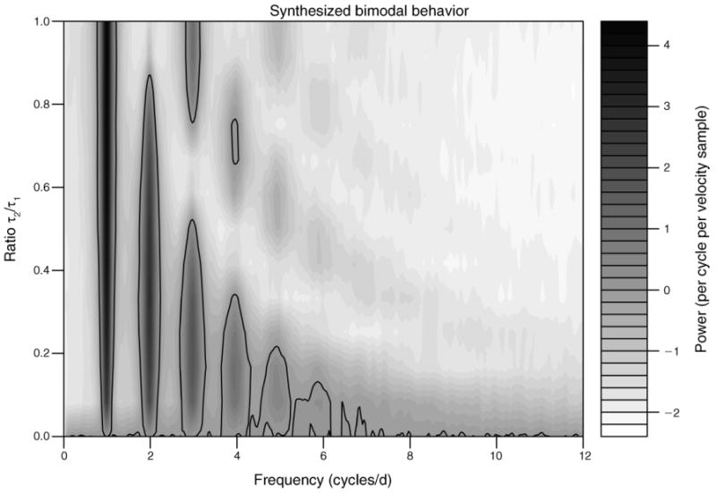
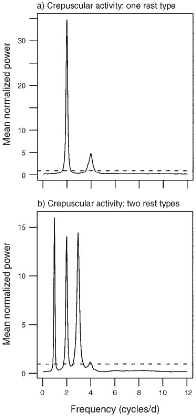
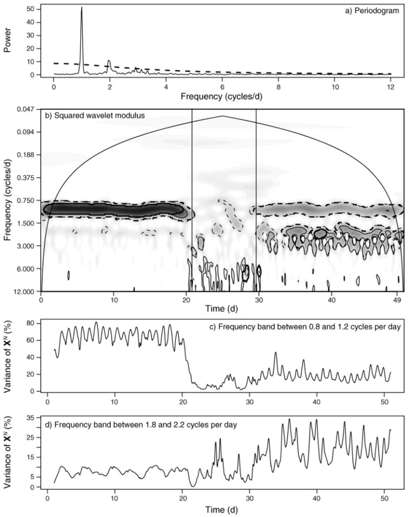
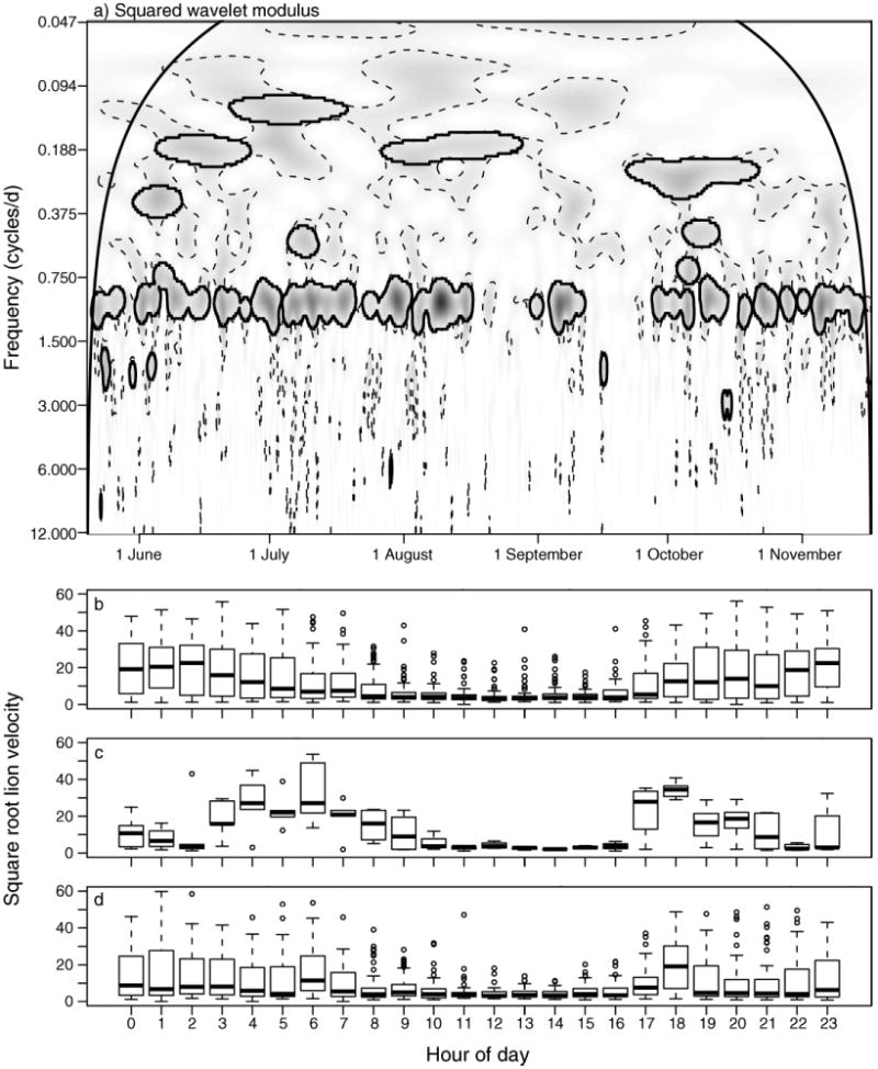
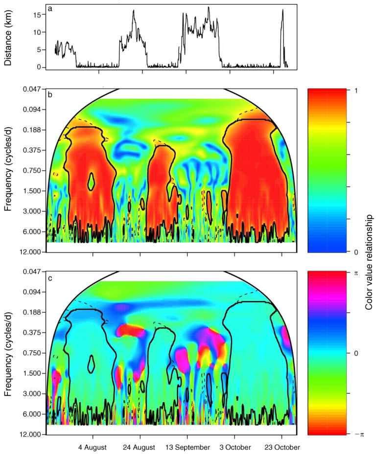
High-resolution animal location data are increasingly available, requiring analytical approaches and statistical tools that can accommodate the temporal structure and transient dynamics (non-stationarity) inherent in natural systems. Traditional analyses often assume uncorrelated or weakly correlated temporal structure in the velocity (net displacement) time series constructed using sequential location data. We propose that frequency and time-frequency domain methods, embodied by Fourier and wavelet transforms, can serve as useful probes in early investigations of animal movement data, stimulating new ecological insight and questions. We introduce a novel movement model with time-varying parameters to study these methods in an animal movement context. Simulation studies show that the spectral signature given by these methods provides a useful approach for statistically detecting and characterizing temporal dependency in animal movement data. In addition, our simulations provide a connection between the spectral signatures observed in empirical data with null hypotheses about expected animal activity. Our analyses also show that there is not a specific one-to-one relationship between the spectral signatures and behavior type and that departures from the anticipated signatures are also informative. Box plots of net displacement arranged by time of day and conditioned on common spectral properties can help interpret the spectral signatures of empirical data. The first case study is based on the movement trajectory of a lion (Panthera leo) that shows several characteristic daily activity sequences, including an active-rest cycle that is correlated with moonlight brightness. A second example based on six pairs of African buffalo (Syncerus caffer) illustrates the use of wavelet coherency to show that their movements synchronize when they are within approximately 1 km of each other, even when individual movement was best described as an uncorrelated random walk, providing an important spatial baseline of movement synchrony and suggesting that local behavioral cues play a strong role in driving movement patterns. We conclude with a discussion about the role these methods may have in guiding appropriately flexible probabilistic models connecting movement with biotic and abiotic covariates.

Fig. 1

Square-root transformed lion (Panthera leo) velocity (m/h before transformation) shown (a) as a time series and (b) as box plots of velocity by time of day where the thick line denotes the median value, the box extends from the 25th to the 75th percentiles, and the whiskers extend to 1.5 times this interquartile range. (c) Fourier periodogram normalized so that the theoretical white-noise spectrum is at the constant power value of 1; the theoretical spectrum of a red-noise data model is shown by the dashed line. The strong peak at 1 cycle/day reflects an overall daily behavioral sequence of resting during the day with increased activity at night. For comparison with time domain methods, panel (d) shows the estimated autocorrelation function (ACF), with the horizontal lines drawn at $\pm 1.96/\sqrt{\mathit{\text{N}}-1}$ corresponding to the approximate 95% confidence intervals for a white-noise data model.

Fig. 2

Contour plot of log_e-transformed, averaged normalized periodogram values (power) from 100 simulated movement trajectories consisting of daily bimodal behavior. The daily behavioral sequence is given by the movement mode set S_K = {m₂, m₃} with the values of m_i as defined in Methods: Stochastic movement model. The expected time spent in mode 2 was varied among {0, 1, …, 12} to span a movement complexity of no behavioral switching (τ₂ = 0, i.e., a random walk), to evenly partitioned switching (τ₂ = τ₁ = 12 hours, i.e., symmetric bimodal behavior). For each ratio we simulated 100 continuous movement paths and sampled locations each hour for 30 days. Lines are contoured at the levels of log_e(1) = 0 and enclose regions of frequencies with power larger than that expected by white noise. S_K is the number of distinct movement modes; m₂ is movement mode 2, and m₃ is movement mode 3, as defined in Methods: Stochastic movement models; τ₁ and τ₂ are expected temporal durations for m₁ and m₂, respectively. Grayscale units are in power per cycle per velocity sample, where power is the periodogram value.

Fig. 3

Periodograms for two kinds of simulated crepuscular activity sampled every hour. (a) For the “one rest type” activity, the daily behavioral sequence was defined by S_K = {m₁, m₃, m₁, m₃} and E_K = {4, 8, 4, 8} (the expected temporal durations for each movement mode m_ik) interpreted as alternating between rest and taxis. (b) The “two rest types” activity was defined by S_K = {m₁, m₃, m₂, m₃} and E_K = {4, 4, 12, 4}, interpreted as the sequence rest, taxis, feed, taxis. The power spectrum in each figure panel represents the mean of 100 normalized periodograms. Horizontal dashed lines are drawn at the value of a theoretical white-noise spectrum.

Fig. 4

Frequency and time–frequency analyses of a simulated individual movement trajectory over 50 days sampled at Δt = 1 hour. The daily behavioral sequence (with m_i defined in Methods: Stochastic movement model) was S_K = {m₁, m₂, m₃, m₂} and E_K = {6, 6, 6, 6}, corresponding to equal times of rest, feed, taxis, feed for the first 20 days, followed by randomly chosen behavioral modes with expected temporal duration τ_k = 1 hour for the middle 10 days, and ending with crepuscular activity defined as S_K = {m₁, m₃, m₂, m₁, m₂, m₃} with E_K = {4, 4, 4, 4, 4} corresponding to equal expected durations of rest, taxis, walk, rest, walk, taxis, during the final 20 days. (a) The normalized smoothed periodogram shows peaks different from white (constant value of 1) or red (dashed line) noise null models, suggesting cyclic behavior. (b) Contoured squared wavelet modules values (smaller values are given by whiter colors and larger values by darker colors). Using 1000 simulated step-length time series based on the white and red noise null models, we calculated the bootstrapped 95th percentile significant patches, delineated by thin dashed and solid lines, respectively; significant patches remaining from an areawise test (see Methods: Fourier and wavelet transformation) are delineated by thick dashed and solid lines for the white and red noise null models, respectively. The cone of influence is delineated by the arched solid black line. Panels (c) and (d) show the time series of the percentage variance explained by frequency bands around (c) ω = 1 cycle/day and (d) ω = 2 cycles/day, where X^N is the length N time series of movement velocities, defined in Methods: Fourier and wavelet transforms.

Fig. 5

(a) Wavelet analysis of lion velocity data (smaller values are given by lighter colors and larger values by darker colors) shows a dominant, yet transient, 1, 2, or no cycles/day behavior. Significant patches are defined as those that lie inside the solid black closed lines, which delineate patch area remaining from an areawise test of patches defined by 95th estimated percentiles obtained from 1000 bootstrapped white-noise null-model time series, delineated by dashed lines. The cone of influence is delineated by the smooth, arched solid black line. (b–d) Tukey box plots, where the thick line denotes the median value, the box extends from the 25th to the 75th percentiles, and the whiskers extend to 1.5 times this interquartile range, of square-root transformed velocity (m/h before transformation) grouped by hour of day for different partitions of the data: (b) times during which scalogram values at 1 cycle/day are significant and explain a greater proportion of the variance than scalogram values at 2 cycle/day, indicating a basic active–rest cycle; (c) times during which scalogram values at 2 cycles/day are significant and explain a greater proportion of the variance than scalogram values at 1 cycle/day, identifying several active nights during which a secondary rest period occurs; (d) box plots without significant scalogram values at 1 or 2 cycles/day, identifying nights with less activity.

Fig. 6

Analyses of two African buffalo (Syncerus caffer; T12 and T13 in Table 1) in July through October 2005: (a) the distance between them, (b) their wavelet coherency, and (c) wavelet coherency phase differences, where the color-value relationship is shown by the color bars to the right of each contour. Wavelet coherence values <1 indicate uncorrelated noise, a nonlinear relationship between the velocity of T12 and T13, or that the processes influencing T12's or T13's velocity are not identical. In panels (b) and (c), significant patches are defined as those that lie inside the solid black closed lines, which delineate patch area remaining from an areawise test of patches defined by 95th estimated percentiles obtained from 1000 bootstrapped white-noise null-model time series, delineated by dashed lines, while the cone of influence is delineated by the smooth, arched solid black line.

References

1. Anderson-Sprecher R, Ledolter J. State–space analysis of wildlife telemetry data. Journal of the American Statistical Association. 1991;86:596–602.
1. Bartumeus F, Da Luz MGE, Viswanathan GM, Catalan J. Animal search strategies: a quantitative random-walk analysis. Ecology. 2005;86:3078–3087.
1. Blatter C. Wavelets. A primer. A. K. Peters; Natick, Massachusetts, USA: 1998.
1. Bovet P, Benhamou S. Spatial-analysis of animals' movements using a correlated random-walk model. Journal of Theoretical Biology. 1988;131
1. Brillinger DR. Simulating constrained animal motion using stochastic differential equations. In: Athreye K, Majumdar M, Puri M, Waymire E, editors. Probability, statistics, and their applications: papers in honor of Rabi Bhattacharya. Lecture Notes in Statistics 41. Institute of Mathematical Statistics; Beachwood, Ohio, USA: 2003. pp. 35–48.
Publication types
LinkOut - more resources