. 2010 May 28:11:291.
doi: 10.1186/1471-2105-11-291.

Washing scaling of GeneChip microarray expression

Affiliations

Washing scaling of GeneChip microarray expression

Hans Binder et al. BMC Bioinformatics. .

Abstract

Background: Post-hybridization washing is an essential part of microarray experiments. Both the quality of the experimental washing protocol and adequate consideration of washing in intensity calibration ultimately affect the quality of the expression estimates extracted from the microarray intensities.

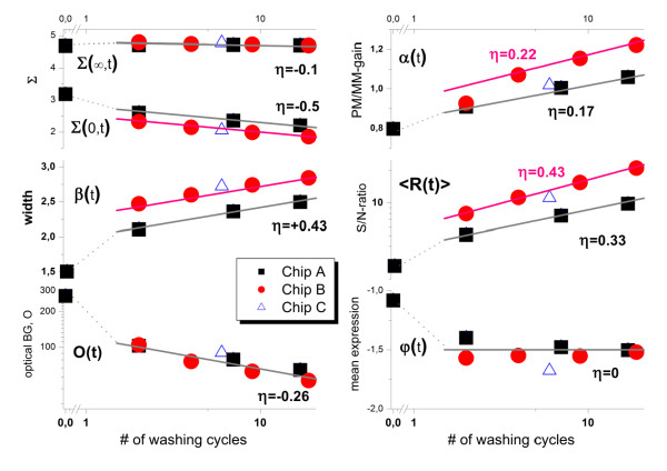
Results: We conducted experiments on GeneChip microarrays with altered protocols for washing, scanning and staining to study the probe-level intensity changes as a function of the number of washing cycles. For calibration and analysis of the intensity data we make use of the 'hook' method which allows intensity contributions due to non-specific and specific hybridization of perfect match (PM) and mismatch (MM) probes to be disentangled in a sequence specific manner. On average, washing according to the standard protocol removes about 90% of the non-specific background and about 30-50% and less than 10% of the specific targets from the MM and PM, respectively. Analysis of the washing kinetics shows that the signal-to-noise ratio doubles roughly every ten stringent washing cycles. Washing can be characterized by time-dependent rate constants which reflect the heterogeneous character of target binding to microarray probes. We propose an empirical washing function which estimates the survival of probe bound targets. It depends on the intensity contribution due to specific and non-specific hybridization per probe which can be estimated for each probe using existing methods. The washing function allows probe intensities to be calibrated for the effect of washing. On a relative scale, proper calibration for washing markedly increases expression measures, especially in the limit of small and large values.

Conclusions: Washing is among the factors which potentially distort expression measures. The proposed first-order correction method allows direct implementation in existing calibration algorithms for microarray data. We provide an experimental 'washing data set' which might be used by the community for developing amendments of the washing correction.


Figures

Figure 1
Figure 1
Workflow of the washing experiment: Three human genome arrays (HG-U133plus2) were hybridized with identical RNA-samples, equilibrated for 16 hours, low stringently washed and stained (labeled) using the same protocol. Stringent wash cycles and subsequent scans were applied using different protocols: Two arrays, A and B, were stringently washed and scanned in four alternating cycles where in each cycle the washing step was repeated several times as indicated. Chip C was processed using the standard protocol of six stringent washes before staining. The chip measurements are assigned according to 'chip-cycle number-(total number of washings)', e.g. A-3(7x). After finishing the first series of wash/scan-cycles the whole procedure was repeated a second time.
Figure 2
Figure 2
PM- and MM-probe intensities of four selected probe sets before (t = 0) and after (t = 17) washing: Each probe set contains eleven PM and MM probes. Washing affects the different probes in a selective fashion. For example, the high-intensity PM-probes a and b (see labels in the figure) remain nearly unaffected, wheras the weak-intensity probes c and d respond strongly to washing. The horizontal dashed lines are the mean intensities which are log-averaged over all eleven probes of each probe set. The figure shows probes with relatively large set-averaged intensities which are predominantly hybridized with specific transcripts. The sequences of the four labeled probes (a-d) are explicitly given together with the total number of adenines, cytosines, guanines and thymines per sequence. Note that there are no obvious correlations between the given sequences and the intensity changes owing to washing.
Figure 3
Figure 3
Probe intensity distributions before (t = 0) and after (t = 17 cycles) washing: Thick and thin lines refer to PM- and MM-probes of chip A, respectively. The different panels show the distributions of: (a) all probes of the array (~6·105 probes), (b) probes predominantly hybridized with non-specific transcripts (2·105 probes) and (c) probes predominantly hybridized with specific transcripts (2·104 probes). Accordingly, about 4·105 probes are not considered because they are significantly hybridized by non-specific and specific transcripts as well. Panel d shows the respective distributions of set-averaged log-intensities. The vertical dotted line at the right indicates the maximum intensity M referring to complete saturation of the probe spots.
Figure 4
Figure 4
Probe intensities as a function of the number of washing cycles: Part a: The probes of three probe sets were selected for large (top row), intermediate (middle row) and low (bottom row) intensity levels (array A; see also Figure 1). The thick lines are the log-mean values averaged over the eleven probes of each probe set. The intensities of PM- and MM-probes and of their log-difference are shown from left to the right as indicated in the figure. Part b re-plots the averaged intensity data of the PM and MM shown in part a after normalization assuming a common start value of w(0) = 1 (symbols). The curves are calculated using Eq. (8).
Figure 5
Figure 5
Limiting values (panel a) and decay times (panel b) of the washing function as a function of the initial probe intensity logIP(0): The dots are the probe-level data of all PM-probes of array A (see Eqs. (8) and (9)). The moving average was calculated over 1000 probe-level data to extract the mean effect of intensity on both parameters (thick curves). The moving average of the MM probes (probe-level data are omitted for clarity) is virtually indistinguishable from that of the PM probes. The PM-data are also split into probes which are hybridized predominantly non-specifically and specifically (thin lines, see text). The respective moving averages cover the low-intensity and high intensity ranges, respectively, with considerable overlap (see arrows in panel a). These results show that the washing parameters are mainly determined by the probe intensities and thus by the binding constant independently of the probe type (PM or MM) and of the hybridization mode (specific or non-specific). The mean trends of w∞ and τ are well described using Eqs. (18) and (17) given in the Methods-section (dashed lines). Accordingly, the stepwise change of the washing parameters is governed by their power law dependence on the binding constant. The fits use a critical exponent of γ = 1.6 and the critical intensities of logI(0)crit = 3.8 (for w∞) and 3.5 (for τ). The critical exponent and the critical intensity determine the sharpness of the sigmoidal change and the position of its inflection point, respectively (see also Figure 16 for illustration).
Figure 6
Figure 6
PM- and MM-characteristics of washing: Mean probe intensity (panel a), the asymptotic washing level (panel b) and the initial washing decay time (panel c) are shown as a function of the set-averaged probe intensity, Σ, which roughly estimates the expression level of the respective probe set. All values are separately calculated for PM and MM probes. Their characteristics are essentially identical upon non-specific hybridization at small Σ-values. Beyond a threshold the data split into two branches due to the onset of specific hybridization. Washing removes specific transcripts more strongly from the MM owing to their weaker binding caused by their central mismatch.
Figure 7
Figure 7
Hook representation of the washing parameters: The figure shows the PM/MM-difference plot of the smoothed intensities before washing (Δ(t = 0) = logIPM/IMM), of the asymptotic washing level (Δw = log(w∞PM/w∞MM)) and of the decay times (Δτ = -(τ PM - τ MM)) as a function of the mean intensity, Σ. These hook plots reveal the typical hybridization regimes: non-specific (N), mixed (mix), specific (S), saturation (sat) and asymptotic (as) as indicated in the figure. The indicated 'percent values' estimate the degree of decrease in terms of the final level compared with the maximum. The dashed curves are theoretical fits using Eq. (20) (Δ(t = 0)) and Eqs. (37)-(38) (Δw), respectively. Note that theory predicts an asymmetric shape of Δw compared with the symmetric shape of Δ(t = 0) in agreement with the experimental curves.
Figure 8
Figure 8
The effect of washing on the Hook-curves: In the second series the chips are labeled and stained a second time and subsequently washed using the same protocol as in the first series. Panel b re-plots the hook-curves for chip A (1 st series) together with theoretical functions which were calculated using Eq. (20) for different numbers of washing cycles. Washing first of all increases the width and the height of the hooks. The two trends reflect different effects: The increased width can be attributed to the strong removal of non-specific transcripts whereas the increased height indicates the stronger effect of washing on the MM-probes. Specific transcripts bound to the PM probes are relatively stable against washing as indicated by the virtually invariant right flank of the hook curves. See also Figure 17 below (part a) which assigns the geometrical dimensions of the hook-curve to the parameters used.
Figure 9
Figure 9
Differential effect of washing between PM and MM probes (part a) and between specific and nonspecific binding (part b): Differences are calculated from the intensities after 17 washing cycles (t = 17) relative to the unwashed chip (t = 0). Panel a illustrates the Δ-coordinates Δ(0) and Δ(17) as a function of the mean intensity Σ(0) and their difference Δ(17) - Δ(0). It shows the typical hook-like shape indicating maximum washing effect on the PM/MM log-intensity difference in the mix-hybridization range. The effect is markedly reduced in the sat- and as-ranges because specific transcripts bind relatively strongly to both PM and MM, strongly reducing their washing efficiency. The PM/MM-ratio of the limiting saturation intensities is given by δαS~0.2 (see also Eq. (28) in the Methods-section). The difference in washing effects virtually disappears in the N-range because the weakly bound nonspecific transcripts are washed off from the PM and MM probes in nearly identical amounts (i.e. δαN~0). Panel b correlates the Σ-coordinates at t = 0 and t = 17. The lower plot shows the difference Σ(17) - Σ(0). The washing effect on the mean intensity is maximum in the N-range (δβN~-0.95, see Eq. (27)). It gradually decreases with increasing contribution of specific hybridization to about δβS~-0.13.
Figure 10
Figure 10
Washing kinetics of the hook-parameters: Hook parameters refer to the studied three chips A, B and C in the first washing series. The kinetic exponent η estimates the slope of the linear fits. The respective values are given in the figure (see Eq. (10)). Chips A and B are scanned at different time points where the first scan of chip A was performed before washing (see Figure 1). Chip C (triangle) refers to the standard washing protocol suggested by the manufacturer. The different chips provide consistent slopes within ± 0.05. The hook parameters are defined in the Methods-section.
Figure 11
Figure 11
Effect of re-labelling of array A on the total intensity distributions of the PM and MM probes (panel a) and on the hook curves (panel b): The data refer to the second scan A2(2x) (see Figure 1). The distributions and hook curves shift to the right after re-labelling as indicated by the grey arrows. This shift applies also to the saturation intensity: M(1st series)→M(2nd series). The latter value exceeds the maximum detectable intensity of the scanner, i.e. Omax < M(2nd). This constraint truncates the intensity distributions at Omax and sets all intensity values greater than the optical limit equal to Omax which causes the small peak at the right end of the distribution. Note that the width of the hooks remains virtually the same in both series whereas its height slightly increases after re-labelling. This result suggests that labelling with SAPE facilitates the washing-off of probe-bound targets. The washing-time kinetics of the hook-parameters is shown in Figure 12.
Figure 12
Figure 12
Washing kinetics of the hook-parameters of the studied three chips before (small symbols) and after (large symbols) re-labeling: The small symbols referring to the first series were re-plotted from Figure 10. The thin dotted lines and the thick lines serve as a guide for the eye to illustrate the trends of the first and second series (chip A), respectively. The respective enrichment factors are given in the right part of the figure (see also Figure 13). The intensity-related parameters Σ(∞,t), Σ(0,t) and O(t) shift to larger values after re-labelling whereas the width of the hook β(t) roughly agrees in both series. The vertical shift between the levels of mean expression φ(t), the mean S/N-ratio <R(t)> and also the PM/MM-gain α(t) reflect the enrichment in the second series as predicted by the simple model illustrated in Figure 13 (the numbers in the right part are the respective enrichment factors, see text).
Figure 13
Figure 13
Schematic illustration of the effect of washing of the microarray using two rounds of staining and washing: The different steps are characterized as follows: Hybridization: The grey areas refer to the amount of PM and MM probe oligomers occupied with specific (S) and nonspecific (N) transcripts (see Eq. (1)). Both probe types are assumed to hybridize identically with non-specific transcripts (P-N, P = PM,MM). Free probe oligomers are not shown. 1st staining: A certain fraction of bound transcripts becomes 'bright' by labeling with fluorescent markers (SAPE) whereas the remaining non-labeled fraction remains 'dark'. The amount of bright probe duplexes of each type in this first labeling round is set to 100%. 1st washing: Washing removes bound targets of the bright fraction from the probes as indicated by the arrows (Eq. (4)). The yield of washing depends on the duplex type: The percentage of reduction of bound targets is largest for nonspecific transcripts and smallest for specific transcripts bound to PM probes. The dark fraction is not affected by washing. 2nd staining: We assume that in the second staining round the same amount of dark probes is transferred into bright ones by labeling as in the first round. The given percentages refer to the amount of bright probes relative to the initial level after 1st staining. For example, the amount of bright PM-S duplexes nearly doubles from 90% to 100%+90% = 190%. 2nd washing: The amount of bound targets reduces by the same duplex-specific factor as in the 1st washing round. For example, 90% of the 190% bright PM-S remain bound (0.9·190% = 171% of the initial level). Note that each staining/washing round enriches high-affinity bright duplexes compared with low-affinity bright ones, e.g. PM-S compared with MM-S and with P-N as indicated in the graph in the upper part of the figure. The given enrichment factors for the expression degree PM-S and the ratios PM-S/MM-S and PM-S/PM-N refer to the second round compared with the first one (see text). Note that the respective hook parameters are related logarithmically to the enrichment factors.
Figure 14
Figure 14
Positional sensitivity profiles of specific (panel a) and non-specific (panel c) hybridization before (t = 0, thick curves) and after (t = 17, thin dashed curves) washing: The respective nucleotide-letters are given in the figure. The respective sensitivity terms estimate the mean contribution of the selected nucleotide at the given position to the observed intensity-increment with respect to the set-mean of the intensity (log-scale, see Eq. (41)). The two panels below (b and d) show the difference profiles 'washed-unwashed'. In addition to the single-base terms we also show nearest-neighbor (NN) terms of selected homo-couples (dotted curves, the original NN-profiles in the upper panels are omitted for clarity). The difference profiles estimate the mean relative stability of the respective nucleotide-letter at the given position against washing. Note that sequence position k = 1 faces towards the bulk solution whereas position k = 25 is attached to the chip-surface.
Figure 15
Figure 15
Systematic bias of 'Langmuir'-expression estimates (Eq. (12)) with respect to the estimates which consider washing (Eq. (11)): Part a and b: Correlation plot between both estimates and their logged difference, formula image
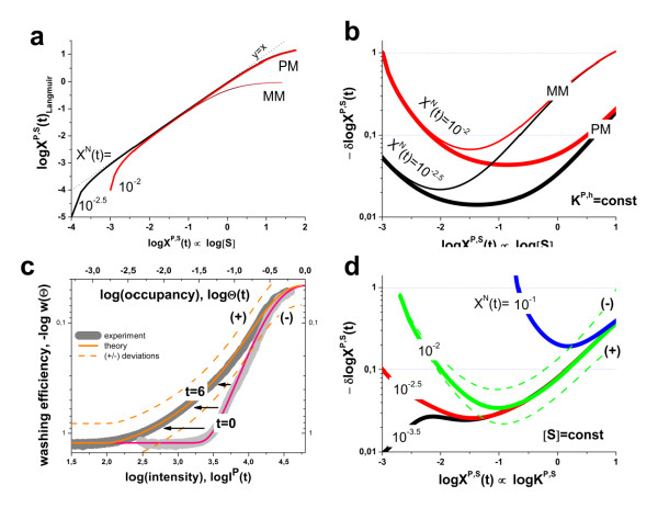
. The graphs were calculated assuming KP,h = const for two non-specific background levels (red and black curves) and for PM and MM probes (dotted and solid curves) assuming the survival fractions wPM,S(t) = 0.95, wMM,S(t) = 0.50 and wP,N(t) = 0.1. Neglecting washing underestimates the expression degree especially at small and large expression values. Part c: The survival fraction of bound probes depends on the intensity (or, equivalently, probe occupancy) before (t = 0) and after washing (t > 0). The graph for t = 0 was re-plotted from Figure 5a using Eq. (17) with wmax = 0.9, wmin = 0.06, γ = 1.6 and a' = 0.1. The graph for t = 6 refers to the standard number of washing cycles. It is obtained from the t = 0 graph by making the substitution logI(t) = logI(0)+log(w(t)) in the argument (see Eq. (8)). Part d shows the bias of the Langmuir approximation assuming a constant transcript concentration and variable KP,S and thus a variable survival fraction w(Θ) which has been taken from part c of the figure for t = 6. The dashed curves labelled with '(+)' and '(-)' in panels c and d refer to 50%-deviations of the washing function, log w(Θ)+/- = log w(Θ)·(1.5)(+/-)1, to estimate the effect of the scattering of the probe level data from the mean (compare with Figure 5a). The bias of the Langmuir-approximation strongly resembles that shown in part b. Note that the bias applies to PM and MM probes as well in this case.
Figure 16
Figure 16
Sigmoidal "switch"-function governed by the exponential power law of the binding constant (Eq. (16)): The "switch"-functions are used to describe the intensity-dependence of the asymptotic washing level and the characteristic decay time (Eq. (18), see also Figure 5). The parameters "switch" between their minimum and maximum values at the characteristic intensity Icrit≈a'M. It depends on the number of washing cycles used for parameter estimation (see Eqs. (17) and (18)). The limiting decay times are given by τmin = 2/ln(wmin(2)) and τmax = 2/ln(wmax(2)) (see Eqs. (18) and (17)). The sharpness of the step is governed by the exponent γ (see figure).
Figure 17
Figure 17
Concentration dependence and hook representation of the washing effect: Part a and b: PM- and MM-probe intensities before (t = 0) and after (t > 0) washing (part a) and the respective hook plots (part b, Eq. (20)). The initial intensities in the limit of small and large specific transcript concentrations decrease by the 'survival' factors wP,h(t) (P = PM,MM; h = N,S) after washing. These trends transform into a 'deformation' and shift of the hook curve: Washing increases its the height (α) and the width (β) by the increments δα≈δαS and δβ = δβS+δβN, respectively (see Eqs. (23), (27) and (28)). The 'start' (R = 0) and 'end' (R = ∞) coordinates are indicated in the figure. The dashed curve is the 'standard' hook approximation (Eq. (30)). Part c and d: Occupancies of the PM- and MM-probes before washing and the respective limiting survival fractions (part c) and the respective log-intensity hook (Δ(t = 0), Eqs. (19) and (20)) and hook-presentation of the asymptotic washing level (Δw(R,∞), Eqs. (37) and (38); part d). Note the asymmetric shape of the latter curve and its limiting height at R→∞ (Eq. (39)). The height-parameters αw and α are related to different hybridization characteristics, namely the non-specific binding strength and the PM/MM-gain, respectively (see text).

Similar articles

Cited by

References

    1. Lipshutz RJ, Fodor SPA, Gingeras TR, Lockhart DJ. High density synthetic oligonucleotide arrays. Nat Genetics. 1999;21:20–24. doi: 10.1038/4447. - DOI - PubMed
    1. Han T, Melvin C, Shi L, Branham W, Moland C, Pine PS, Thompson K, Fuscoe J. Improvement in the Reproducibility and Accuracy of DNA Microarray Quantification by Optimizing Hybridization Conditions. BMC Bioinformatics. 2006;7(Suppl 2):S17. doi: 10.1186/1471-2105-7-S2-S17. - DOI - PMC - PubMed
    1. Pozhitkov AE, Stedtfeld RD, Hashsham SA, Noble PA. Revision of the nonequilibrium thermal dissociation and stringent washing approaches for identification of mixed nucleic acid targets by microarrays. Nucl Acids Res. 2007;35(9):e70. doi: 10.1093/nar/gkm154. - DOI - PMC - PubMed
    1. Skvortsov D, Abdueva D, Curtis C, Schaub B, Tavare S. Explaining differences in saturation levels for Affymetrix GeneChip(R) arrays. Nucl Acids Res. 2007;35(12):4154–4163. doi: 10.1093/nar/gkm348. - DOI - PMC - PubMed
    1. Wick L, Rouillard J, Whittam T, Gulari E, Tiedje J, Hashsham S. On-chip non-equilibrium dissociation curves and dissociation rate constants as methods to assess specificity of oligonucleotide probes. Nucl Acids Res. 2006;34(3):e26. doi: 10.1093/nar/gnj024. - DOI - PMC - PubMed

Publication types

MeSH terms