. 2010 Jun;63(6):1583-93.
doi: 10.1002/mrm.22381.

Quantitative sodium imaging with a flexible twisted projection pulse sequence

Affiliations

Quantitative sodium imaging with a flexible twisted projection pulse sequence

Aiming Lu et al. Magn Reson Med. 2010 Jun.

Abstract

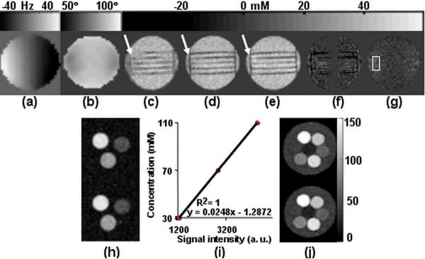
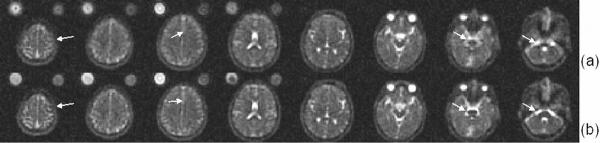
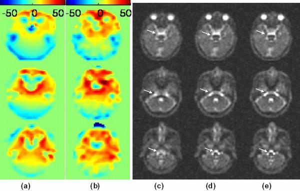
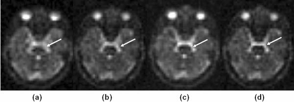
The quantification of sodium MR images from an arbitrary intensity scale into a bioscale fosters image interpretation in terms of the spatially resolved biochemical process of sodium ion homeostasis. A methodology for quantifying tissue sodium concentration using a flexible twisted projection imaging sequence is proposed that allows for optimization of tradeoffs between readout time, signal-to-noise ratio efficiency, and sensitivity to static field susceptibility artifacts. The gradient amplitude supported by the slew rate at each k-space radius regularizes the readout gradient waveform design to avoid slew rate violation. Static field inhomogeneity artifacts are corrected using a frequency-segmented conjugate phase reconstruction approach, with field maps obtained quickly from coregistered proton imaging. High-quality quantitative sodium images have been achieved in phantom and volunteer studies with real isotropic spatial resolution of 7.5 x 7.5 x 7.5 mm(3) for the slow T(2) component in approximately 8 min on a clinical 3-T scanner. After correcting for coil sensitivity inhomogeneity and water fraction, the tissue sodium concentration in gray matter and white matter was measured to be 36.6 +/- 0.6 micromol/g wet weight and 27.6 +/- 1.2 micromol/g wet weight, respectively.


Figures

Figure 1
Figure 1
An illustration of k-space sampling strategy of TPI in which each trajectory has a radial component arising at the center of k-space and extending to K0 along a cone of angle θ, and then twisting along the surface of the cone to reach the maximum value Kmax. Each trajectory is rotated around the cone to fully sample its surface. Both positive and negative trajectories are acquired.
Figure 2
Figure 2
(a) Illustration of the data acquisition steps. (b) Flow chart of the image reconstruction and quantification processes. The eddy current correction data can be collected beforehand on 1H data, assuming the 1H and the 23Na coils have the same eddy current characteristics.
Figure 3
Figure 3
(a) Typical gradient waveforms designed with the flexTPI scheme (solid lines) and the original TPI scheme with readout gradient amplitude supported by the slew rate (dotted lines) and gradient amplitude higher than that supported by the slew rate (dashed lines). (b) Total slew rate curves corresponding to the waveform designs in (a). The horizontal line at 15,000G/cm/s denotes the maximum hardware slew rate.
Figure 4
Figure 4
(a) Measured gradient waveforms for flexTPI on three axes during the acquisition time. (b) k-space deviation from the nominal trajectories due to linear eddy currents during the acquisition time. (c) Accumulated phase due to B0 eddy currents during the acquisition time. Representative axial images of a high-resolution phantom demonstrate the effects of deviations between the start of the ADC readout and the response of the gradient drivers producing the gradient waveforms: (d) timing error of 16 microseconds, (e) no timing error, and (f) no timing error and with eddy current correction.
Figure 5
Figure 5
Representative coronal images showing the effectiveness of B0 and B1 field inhomogeneity correction. (a) B0 field maps in Hz show a gradient extending from ~−50 Hz to +50 Hz along the z-direction. (b) B1 maps show sensitivity falloff toward the end of the coil. (c) TSC maps without correction (d) TSC maps with B0 correction. (e) TSC maps with both B0 and B1 correction. (f) Difference images ((d) – (c)) showing the effectiveness of B0 inhomogeneity correction. (g) Difference images ((e) – (d)) showing the impact of B1 inhomogneity correction. The improvement in image quality can be clearly appreciated, as shown by the arrows and near the rods with B0 inhomogeneity correction. More homogeneous TSC has been obtained with B1 correction, especially along z-axis need the edges of the phantom. (h) Representative axial images of the calibration phantom containing three different sodium concentrations made in agar gel. (i) Linear calibration curve derived from the calibration phantom. (j) Representative axial images a phantom containing seven different vials filled NaCl solutions of concentrations range from 19.3 mM to 154 mM (19.3, 38.5, 57.8, 77.0, 115.5, 134.8, 154 mM). The acquisition time for sodium imaging was 13 minutes with a nominal isotropic resolution of 5 mm.
Figure 6
Figure 6
Representative axial sodium images of a normal volunteer showing the effectiveness of B0 field inhomogeneity correction. (a) Uncorrected sodium images. (b) Corrected sodium images. The improvement in image quality can be appreciated in the brainstem and orbital frontal regions, as shown by the arrows. The acquisition time was 8 minutes with a nominal isotropic resolution of 4.4 mm.
Figure 7
Figure 7
Axial B0 field maps are shown for a normal volunteer using (a) sodium imaging in 4 minutes and (b) proton imaging in less than 2 minute. These B0 maps were applied to (c) the uncorrected images to derive (d) human images corrected using sodium B0 field maps and (e) human images corrected using proton B0 field maps. The improvements, appreciated in the brainstem (white arrows), are similar for both sodium and proton B0 maps.
Figure 8
Figure 8
Axial sodium images acquired (a) with readout lengths of 28 ms (a) without B0 correction and (b) with B0 correction, and with readout length of 14 ms (c) without B0 correction and (d) with B0 correction. The shorter readout time with B0 correction (d) produces the least blurring of the brainstem (white arrow).
Figure 9
Figure 9
Representative tissue sodium concentration maps (a) obtained on a healthy volunteer (unit: mmol/L tissue). The corresponding T1 weighted proton images are also shown (b) as anatomical references. The TSC images shown are before water fraction correction. The white matter is predominately shown in light blue, while the gray matter is recognized as green between CSF (shows as yellow to dark red due to partial volume effects with brain parenchyma) and white matter.
Figure 10
Figure 10
Simulated point-spread-functions (PSF) for sodium imaging with flexTPI for two typical T2 values of 2ms and 15ms representing the fast and slow components, respectively. The acquisition parameters of the sequence used for the simulation are the same as those used in the consistency study. The PSFs are scaled to the same maximum peak amplitude. The fast component has a broader peak and, therefore, corresponds to a lower spatial resolution. The side lobes are due to zero padding used during the PSF generation.

Similar articles

Cited by

References

    1. Skou J. The influence of some cations on an adenosine triphosphatase from peripheral nerves. Biochim Biophys Acta. 1957;23:394–401. - PubMed
    1. Lodish HF. Molecular cell biology. Scientific American Books; New York: 1999. p. 973.
    1. Thulborn KR, Davis D, Snyder J, Yonas H, Kassam A, Sodium MR. Imaging of Acute and Subacute Stroke for Assessment of Tissue Viability. Neuroimag Clin N Am. 2005;15:639–653. - PubMed
    1. Thulborn KR, Gindin TS, Davis D, Erb P. Comprehensive MRI Protocol for Stroke Management: Tissue Sodium Concentration as a Measure of Tissue Viability in a Non-Human Primate Model and Clinical Studies. Radiology. 1999;139:26–34. - PubMed
    1. Goldsmith M, Damadian R. NMR in cancer. Physiol Chem Phys. 1975;7:263–269. - PubMed

Publication types