

Optimal hierarchical modular topologies for producing limited sustained activation of neural networks
- PMID: 20514144
- PMCID: PMC2876872
- DOI: 10.3389/fninf.2010.00008
Optimal hierarchical modular topologies for producing limited sustained activation of neural networks
Abstract
An essential requirement for the representation of functional patterns in complex neural networks, such as the mammalian cerebral cortex, is the existence of stable regimes of network activation, typically arising from a limited parameter range. In this range of limited sustained activity (LSA), the activity of neural populations in the network persists between the extremes of either quickly dying out or activating the whole network. Hierarchical modular networks were previously found to show a wider parameter range for LSA than random or small-world networks not possessing hierarchical organization or multiple modules. Here we explored how variation in the number of hierarchical levels and modules per level influenced network dynamics and occurrence of LSA. We tested hierarchical configurations of different network sizes, approximating the large-scale networks linking cortical columns in one hemisphere of the rat, cat, or macaque monkey brain. Scaling of the network size affected the number of hierarchical levels and modules in the optimal networks, also depending on whether global edge density or the numbers of connections per node were kept constant. For constant edge density, only few network configurations, possessing an intermediate number of levels and a large number of modules, led to a large range of LSA independent of brain size. For a constant number of node connections, there was a trend for optimal configurations in larger-size networks to possess a larger number of hierarchical levels or more modules. These results may help to explain the trend to greater network complexity apparent in larger brains and may indicate that this complexity is required for maintaining stable levels of neural activation.
Keywords: brain connectivity; cerebral cortex; functional criticality; modularity; neural dynamics; neural networks.
Figures
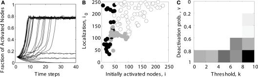
 ), spread through the whole network (o) or was sustained within a limited compartment of the network (
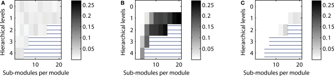
 ). (C) The parameter space of simulations was further explored for different combinations of deactivation probability v and activation threshold k. Gray levels for each parameter combination in the diagram reflect the percentage of cases giving rise to LSA (from subplot B). The average value across all entries was taken as the final measure of the parameter range of LSA for a particular network topology. It reflects the average proportion of limited sustained activation cases obtained across all parameter settings for a given hierarchical modular network.
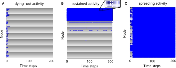
Similar articles
-
Optimal Interplay between Synaptic Strengths and Network Structure Enhances Activity Fluctuations and Information Propagation in Hierarchical Modular Networks.Brain Sci. 2020 Apr 10;10(4):228. doi: 10.3390/brainsci10040228. Brain Sci. 2020. PMID: 32290351 Free PMC article.
-
Sustained activity in hierarchical modular neural networks: self-organized criticality and oscillations.Front Comput Neurosci. 2011 Jun 29;5:30. doi: 10.3389/fncom.2011.00030. eCollection 2011. Front Comput Neurosci. 2011. PMID: 21852971 Free PMC article.
-
Hierarchical modularity in human brain functional networks.Front Neuroinform. 2009 Oct 30;3:37. doi: 10.3389/neuro.11.037.2009. eCollection 2009. Front Neuroinform. 2009. PMID: 19949480 Free PMC article.
-
Detecting hierarchical modularity in biological networks.Methods Mol Biol. 2009;541:145-60. doi: 10.1007/978-1-59745-243-4_7. Methods Mol Biol. 2009. PMID: 19381526 Review.
-
Scaling in Colloidal and Biological Networks.Entropy (Basel). 2020 Jun 4;22(6):622. doi: 10.3390/e22060622. Entropy (Basel). 2020. PMID: 33286394 Free PMC article. Review.
Cited by
-
Link-usage asymmetry and collective patterns emerging from rich-club organization of complex networks.Proc Natl Acad Sci U S A. 2020 Aug 4;117(31):18332-18340. doi: 10.1073/pnas.1919785117. Epub 2020 Jul 20. Proc Natl Acad Sci U S A. 2020. PMID: 32690716 Free PMC article.
-
Selective inhibition of excitatory synaptic transmission alters the emergent bursting dynamics of in vitro neural networks.Front Neural Circuits. 2023 Feb 16;17:1020487. doi: 10.3389/fncir.2023.1020487. eCollection 2023. Front Neural Circuits. 2023. PMID: 36874945 Free PMC article.
-
Hierarchy and dynamics of neural networks.Front Neuroinform. 2010 Aug 23;4:112. doi: 10.3389/fninf.2010.00112. eCollection 2010. Front Neuroinform. 2010. PMID: 20844605 Free PMC article. No abstract available.
-
The role of long-range connectivity for the characterization of the functional-anatomical organization of the cortex.Front Syst Neurosci. 2011 Jul 7;5:58. doi: 10.3389/fnsys.2011.00058. eCollection 2011. Front Syst Neurosci. 2011. PMID: 21779237 Free PMC article.
-
Optimal Interplay between Synaptic Strengths and Network Structure Enhances Activity Fluctuations and Information Propagation in Hierarchical Modular Networks.Brain Sci. 2020 Apr 10;10(4):228. doi: 10.3390/brainsci10040228. Brain Sci. 2020. PMID: 32290351 Free PMC article.
References
-
- Albert R., Barabási A.-L. (2002). Statistical mechanics of complex networks. Rev. Mod. Phys. 74, 47–9710.1103/RevModPhys.74.47 - DOI
LinkOut - more resources
Full Text Sources
Miscellaneous