A three-dimensional atlas of the honeybee neck

Abstract

Three-dimensional digital atlases are rapidly becoming indispensible in modern biology. We used serial sectioning combined with manual registration and segmentation of images to develop a comprehensive and detailed three-dimensional atlas of the honeybee head-neck system. This interactive atlas includes skeletal structures of the head and prothorax, the neck musculature, and the nervous system. The scope and resolution of the model exceeds atlases previously developed on similar sized animals, and the interactive nature of the model provides a far more accessible means of interpreting and comprehending insect anatomy and neuroanatomy.

Figure 1. Orthogonal views of the reconstructed model.

Left column: model with no translucency. Middle column: model with exoskeleton translucent. Right column: only exo- and endo-skeletal components shown. Surface structures partially translucent. (A) Frontal view (minus frons and mouthparts). (B) Side view. (C) Dorsal view. (D) Ventral view. Cx: coxa of the foreleg; DNM: dorsal neck membrane; H: head; Pn: pronotum; Pp: propectus; Mn: mesonotum. D: dorsal; V: ventral; L: lateral; A: anterior; P: posterior.

Figure 2. The head and propectuses.

(A) Oblique frontal view. (B) Posterior view of the head. (C) Enlarged view of the foramen magnum and surrounding structures. (D) Articulation of the right propectus with the head (left propectus not shown). (E) Posterolateral view. (F) Dorsal view including the endosternum. White arrow marks a protruding flange that may prevent over-protraction of the propectus. FM: foramen magnum; OC: occipital condyles; PC; propectal condyle; PGL: postgenal lobes; PPl: pleural plate of propectus; SPl: sternal plate of prospectus; TP: tentorial pits. Colour codes as in Fig. 1.

Figure 3. The endosternum.

(A) Frontal view of endosternum and propectus. (B) Lateral view of endosternum, right propectus and right fore coxa. (C) Posterior view of endosternum, propectuses and fore coxae. (D) Oblique posterodorsal view of endosternum, propectuses, coxae and dorsal neck membrane. NF: neural foramen; Colour codes and labels as in Fig. 1.

Figure 4. The pronotum, mesonotum and dorsal neck membrane (DNM).

(A) Anterior view of skeletal structures of the prothorax. (B) Same as (A), posterior view. (C) Same as (A), lateral view. Pronotum not shown to expose the prephragma, first phragma and DNM. (D) Enlarged posterior view of pronotum and propectus. IM: intersegmental membrane; PPh: prephragma of the mesonotum; 1 Ph: first phragma of the mesonotum; PS: pronotal sulcus. Colour codes and labels as in Fig. 1.

Figure 5. Ventral nerve cord (VNC) and nerves innervating the neck muscles; IK1, IK2 and IN1.

(A) Dorsal view of brain, VNC and nerves. Arrow marks where IN1 meets IN6. (B) Posterodorsal view of nervous system with surrounding skeletal structures. Mesonotum shown translucent to expose full extent of IK2. (C) Lateral view of same with only right prospectus and mesonotum (translucent) shown. (D) Enlarged view of nerve cord exiting foramen magnum. For clarity only left IK1, and right IK2 and IN2 are shown. Arrow marks location where IK2 meets IN1. Colour codes and labels as in Fig. 1.

Figure 6. Schematic diagram illustrating direct and indirect head rotation around the three primary axes.

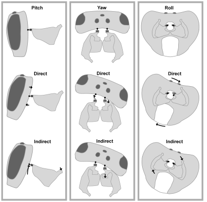
Left: the head and propectus from the side in their natural position, after direct upward head pitch, and after indirect upward head pitch. Middle: the head and prospectus from above in their natural position, after direct rightward head yaw, and indirect rightward head yaw. Right: the head and prospectus as seen from the back in their natural position, after direct rightward head roll, and indirect rightward head roll. In all cases the head is rotated by 20°. Dark grey indicates the occipital processes, filled circles indicate the pivot points of the head.

Figure 7. The direct neck muscles.

(A) Dorsal view of muscles 40a–41b. Pronotum and mesonotum translucent. (B) Posterior view of same showing innervation by IK2. Mesonotum translucent. (C) Side view of right muscle 42a/b/c and right propectus. (D) Oblique posterodorsal view of same showing IN1 innervation. (E) Lateral view of muscles 43 and 44. (F) Dorsal view of left muscle 43 and right muscle 44 showing innervation by left IN1 and right IK1 respectively. Colour codes as in Fig. 1.

Figure 8. The indirect neck muscles.

(A) Anterior view of muscles 45–48. Pronotum and mesonotum translucent. (B) Dorsal view of same. (C) Posterior view of same showing innervation by IN1 (left) and IK2 (right). Mesonotum translucent. (D) Side view of muscles 49–51. Pronotum translucent. (E) Side view of same with overlying pronotum and left propectus not shown. (F) Dorsal view of 49 and 50 (right), and 51a and 51b (left). Innervation by IN1 (right) and IK1 (left) also shown. 49 and 51a shown translucent to expose underlying 50 and 51b, respectively. Colour codes as in Fig. 1.

Figure 9. The leg muscles of the propectus, endosternum and pronotum.

(A) Promoters of the fore coxae: dorsal view; (B) anterolateral view of right propectus, right 53a/b, left 54 and left mcr. (C) Remoters of the fore coxae: dorsal view; (D) Posterior view of right 55, right 56, left 61a (translucent) and left 61b. Colour codes as in Fig. 1.

Figure 10. The steps involved in generation of the three-dimensional atlas.

(A) Imaging: multiple images of each section were stitched together to create a single high-resolution image. Outline of multiple images are visible as white boundaries on the black background. (B) Alignment: images of each section were aligned relative to each other. Registration was quickly verified by volume rendering the image stack; the bee head and thorax are shown from the top (left) and side (right). (C) Segmentation: every structure of interest was manually outlined in each of the aligned sections. Different colours overlaid over this cross-section of the prothorax represent different structures. The boxed area illustrates the region shown in Fig. 11. (D) Model generation: mesh models were created from stacks of segmented images using Amira 3.1. (E) Redrawing: mesh models were greatly smoothed, simplified, and corrected for artefacts by manually redrawing using Silo 2.1. The approximate total number of polygons in each of the mesh models is indicated by n.

Figure 11. Representative image contrast.

(A) Enlarged view of the marked region of section shown in Fig. 10C. The original image before segmentation is shown. Section was taken in a transverse plane, at a level near the anterior margin of the endosternum. The ventral direct neck muscles and their innervating nerves are visible. (B) Histogram of intensity values of the image shown in (A).

References

-
- Odgaard A, Andersen K, Melsen F, Gundersen HJ. A direct method for fast three-dimensional serial reconstruction. J Microsc. 1990;159:335–342. - PubMed
- Weninger WJ, Meng S, Streicher J, Müller GB. A new episcopic method for rapid 3-D reconstruction: applications in anatomy and embryology. Anat Embryol. 1998;197:341–348. - PubMed
- Brandt R, Rohlfing T, Rybak J, Krofczik S, Maye A, et al. Three-dimensional average-shape atlas of the honeybee brain and its applications. J Comp Neurol. 2005;492:1–19. - PubMed
- Kelber C, Rossler W, Kleineidam CJ. Multiple olfactory receptor neurons and their axonal projections in the antennal lobe of the honeybee Apis mellifera. J Comp Neurol. 2006;496:395–405. - PubMed
Publication types
MeSH terms
LinkOut - more resources
Full Text Sources