An expanded set of photoreceptors in the Eastern Pale Clouded Yellow butterfly, Colias erate

Abstract

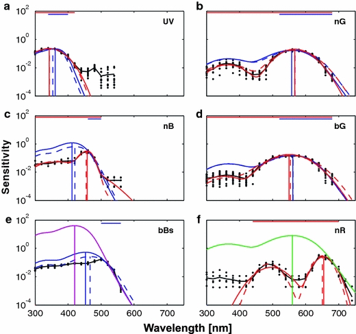
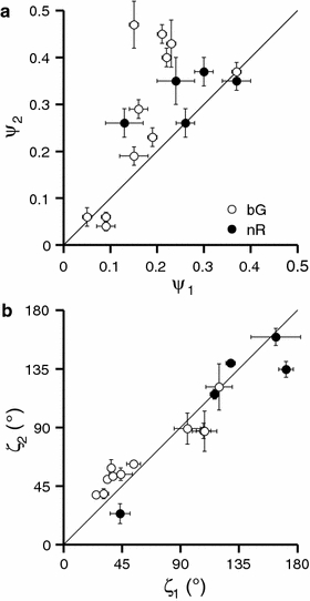
We studied the spectral and polarisation sensitivities of photoreceptors of the butterfly Colias erate by using intracellular electrophysiological recordings and stimulation with light pulses. We developed a method of response waveform comparison (RWC) for evaluating the effective intensity of the light pulses. We identified one UV, four violet-blue, two green and two red photoreceptor classes. We estimated the peak wavelengths of four rhodopsins to be at about 360, 420, 460 and 560 nm. The four violet-blue classes are presumably based on combinations of two rhodopsins and a violet-absorbing screening pigment. The green classes have reduced sensitivity in the ultraviolet range. The two red classes have primary peaks at about 650 and 665 nm, respectively, and secondary peaks at about 480 nm. The shift of the main peak, so far the largest amongst insects, is presumably achieved by tuning the effective thickness of the red perirhabdomal screening pigment. Polarisation sensitivity of green and red photoreceptors is higher at the secondary than at the main peak. We found a 20-fold variation of sensitivity within the cells of one green class, implying possible photoreceptor subfunctionalisation. We propose an allocation scheme of the receptor classes into the three ventral ommatidial types.

Fig. 1

Intracellular recording from a cell classified as a UV receptor. a The sequence starts with a spectral scan of 23 approximately isoquantal light pulses from 300 to 740 nm spaced 20 nm apart. This is followed with a scan going back from 740 to 300 nm. The responses in the green wavelength region are slightly hyperpolarising, possibly due to an ERG artefact or electrical crosstalk from neighbouring green receptors. The intensity calibration scan consists of responses to light pulses at 380 nm, covering an intensity range of 4 log units, increasing in 0.25 log unit steps. The polarisation sensitivity scan was also performed at 380 nm. It starts with five adaptation prepulses, which are followed by 36 pulses with the polariser being rotated in 10° steps. The duration of each of the three protocols was ~40 s. b Estimation of effective intensity of the light pulses. The background waterfall plot shows the root mean square difference (RMSD) profiles (see Fig. 2e, f). The RMSD minima are estimates of effective intensities obtained by the RWC method (black circles). Open squares show the estimates obtained by reverse transformation of a Hill sigmoid

Fig. 2

The response waveform comparison (RWC) method. a, b, c The interpolation of the calibration responses. d, e, f The principle of estimation of effective intensities of the responses. As an example, we estimated the effective intensities of the responses from the same calibration run to perform self-validation of the method. a Measured calibration responses to light pulses with intensity increasing in 0.25 log unit steps over a range of 4 log units (from −4 to 0). The response at logI = −2 is shown in red, and the responses at logI = −4, −3, −1 and 0 are given in blue. The black line marks the shutter opening. b Waterfall plot of the interpolated response array. The measured responses are shown interlaced at their nominal intensities. c Comparison between the measured and interpolated responses. Interpolated responses (spaced 0.05 log unit apart) are shown in black. The measured responses are shown as in a. The inset below the responses shows the difference between the measured and interpolated responses. d Waterfall plot showing the absolute sample-wise difference between the measured response to a light pulse at intensity logI = −2 (red trace in c) and the interpolated response array (shown in b). As expected, the sample-wise difference is close to zero (black colour) in the region around logI = −2. See also the red RMSD profile in e. e RMSD profiles (root mean square sample-wise difference between the measured response and each of the interpolated responses) for some of the calibration stimuli. The positions of the minima of the RMSD profiles were used as the estimators of the effective intensities of the applied stimuli. The red curve presents the RMSD profile for the response to a light pulse at logI = −2 (compare with d). The RMSD minimum for the measured response (0.47 mV) is reached at logI = −2.04 (red circle in e, f). Blue curves, showing the RMSD profiles for the measured responses at logI = −4, −3, −1 and 0, and the black thin curves (responses to intensities at 0.5 log units in between) have their minima close to the applied intensities. f Waterfall plot of the RMSD profiles of all the measured responses from the calibration run. The white crosses, representing the minima of RMSD curves for each stimulus (repeated as solid blue diamonds in Fig. 3), show a close correlation between the applied and estimated intensity (colour figure online)

Fig. 3

Self-validation comparison of the RWC and Hill method. Comparison of the accuracy of the effective stimulus estimation based on retesting the calibration stimuli. The RWC estimates (blue circles, linear regression y = 1.014x + 0.018; thick blue line) are closer to the ideal 1:1 relation between the applied and estimated intensity than the estimates obtained via the inverse Hill transformation (red squares, y = 1.302x + 0.484; thick red line). The Hill sigmoid fit to the intensity–response curve (not shown) was tight, with V _p = 37.0 ± 0.6 mV, logR = −1.65 ± 0.03 and h = 0.75 ± 0.03 (mean ± SE). The red and blue crosses show the estimates obtained from a second intensity–response series (not shown in Fig. 1), compared with the calibration stimuli. The regression lines for these two series are shown with thin blue and red lines. Again, the RWC estimates are closer to 1:1 relation than those obtained from inverse Hill transformation (colour figure online)

Fig. 4

Spectral sensitivities. a Spectral sensitivities of the set of the nine photoreceptor classes of C. erate normalised to their area. The area between the faint lines represents standard deviations. b Spectral sensitivities normalised to the peak, with a logarithmic ordinate. Error bars are omitted here for the sake of clarity. Number of measured cells (n) and individuals (m) for all classes is given as (n, m): UV (13, 9); V (4, 4); nB (6, 6); bBb (6, 5); bBs (6, 3); nG (9, 9); bG (21,10); nR (6, 5), fR (2,2)

Fig. 5

Fits to the sensitivity profiles of UV, nB, bBs, nG, bG and nR classes. The measured log sensitivity spectra (black dots; black line shows the average) were fitted with the rhodopsin templates (blue lines) and heuristic asymmetric Gaussian functions (red lines). The fitting was performed both in the logarithmic (solid lines) and in the linear domain (dashed lines). The vertical lines designate the peak wavelengths obtained with different fits. The horizontal bars designate the interval of data used for fitting the template spectra (blue lines) and heuristic fits (red lines). The UV, nB and bBs sensitivity spectra in the left-hand column (a, c, e) yielded predictions for rhodopsins peaking in the UV, violet and blue, respectively (see Table 1). The magenta line in e, showing the template of a rhodopsin peaking at 420 nm, was fitted by eye. In the right-hand column, the nG and the bG spectra (b, d) yielded predictions for a rhodopsin absorbing maximally at 560 nm (see Table 1). The green line in (f), showing this rhodopsin spectrum, was fitted to the sensitivity profile of the nR class by eye. The numerical fitting results for all classes are shown in Tables 1, 2, and 3. Fits to classes V and bBb are not shown. Individual fits to nR and fR classes are shown in Fig. 10 (colour figure online)

Fig. 6

Analysis of polarisation sensitivities (PS). a Relative polarisation sensitivity amplitudes (ψ). b Angles of maximal polarisation sensitivity (PS axis angles, ζ). The panels are sorted by the receptor class and ζ. Black points represent the estimators ζ ₁ and ψ ₁ measured close to the primary sensitivity peak (380, 420, 460, 500, 560 and 640 nm). Grey points represent the estimators at the secondary sensitivity peak, ζ ₂ and ψ ₂ (380 and 480 nm for the green and red receptor classes, respectively). Thin bars indicate the standard errors of the estimators. Asterisks mark the nB and nG groups, where the polarisation axis estimates are unreliable. Thick bars in a show group averages (±SD) ζ for the receptor classes

Fig. 7

Correspondence of PS amplitude and axis of bG and nR cells. a The relative polarisation sensitivity amplitudes of primary (ψ ₁) and secondary peaks (ψ ₂) of some bG (open circles) and nR cells (solid circles). b The respective PS axis angles (angles of maximal polarisation sensitivity, ζ). Error bars represent standard errors of the estimates. Angles ζ show good correspondence, whilst ψ ₂ is on average bigger than ψ ₁

Fig. 8

Parameters of the intensity–response curve. A scatter plot of the two parameters of the Hill function, V _p (abscissa), and the slope, h (ordinate). Black dots represent estimates for 50 individual cells where the function fit converged well. Solid circles with crosses are group averages (mean ± SD; number of cells in classes: UV 4, V 3, nB 5, bBb 3, bBs 5, bG 18, nG 8, R 4). The thick solid cross is the grand average calculated from individual cells (mean ± SD): V _p = 41.1 ± 6.8 mV and h = 0.73 ± 0.09. The regression line, based on individual cells (h = 0.99 − 0.0064 V _p; r ² = 0.24), shows a weak correlation between a lower maximal response and a steeper slope. The edge histograms show the distributions of the two parameters

Fig. 9

Absorbance difference spectra. The difference between the log sensitivity spectra of the nB and V classes (V – nB) yields a spectrum peaking at ~420 nm as the estimate of the absorbance spectrum of the fluorescing pigment (magenta line with circles). The absorbance difference spectra, calculated as the difference between the rhodopsin template (Rh560) and the spectral sensitivity profiles of nR (red) and fR (black) receptors have peaks (~3 and ~4 log units, respectively) at around 560 nm. The absorbance spectrum of a 5 μm slab of the red pigment (blue line with circles) has been calculated from the thin layer transmittance spectrum measured by Arikawa et al. (2009) under the assumption that the red pigment has negligible absorption at 700 nm. The cyan lines show a simulated effective optical thickness increase of 4.5-, 9- and 18-fold (dotted, dash-dotted and dashed blue lines, respectively). The latter factor has been chosen to fit the LW limb of the absorbance difference spectrum for the nR class (red) (colour figure online)

Fig. 10

Analysis of individual red receptors. a Fits of the sum of double Gaussian functions to the sensitivity profiles of the eight receptors from the red class with the provisional division into the nR subclass (black) and fR subclass (red). Dots show the experimental data. Thin lines show fits to individual cells and thick lines show the fits to the joined data from six nR cells (black) and two fR cells (red). b The relation between the peak position estimates (circles), the left cutoff estimates (WLHM; crosses) and the relative amplitude of the secondary peak at 480 nm (y-axis) (colour figure online)

Fig. 11

Provisional scheme of the three proposed ventral ommatidial types in C. erate. a Only Type I ommatidia fluoresce under violet (<420 nm) excitation. b CeV1 and CeV2 mRNA are co-expressed in R1 and R2 cells of Type I and II ommatidia (Awata et al. 2009). Receptor R9 (always expressing CeL) has been omitted for the sake of clarity. c The size and orientation of arrows depicts the polarisation sensitivity (PS) of the various receptor classes. The relative size of the coloured slabs depicts how much microvilli each receptor class contributes to the rhabdom. Colour coding is consistent with receptor classes in Fig. 4 (colour figure online)

References

1. Arikawa K. Color vision. In: Eguchi E, Tominaga Y, editors. Atlas of arthropod sensory receptors. Tokyo: Springer-Verlag; 1999. pp. 23–32.
1. Arikawa K. Spectral organization of the eye of a butterfly, Papilio. J Comp Physiol A. 2003;189:791–800. doi: 10.1007/s00359-003-0454-7. - DOI - PubMed
1. Arikawa K, Stavenga DG. Random array of colour filters in the eyes of butterflies. J Exp Biol. 1997;200:2501–2506. - PubMed
1. Arikawa K, Uchiyama H. Red receptors dominate the proximal tier of the retina in the butterfly Papilio xuthus. J Comp Physiol A. 1996;178:55–61. doi: 10.1007/BF00189590. - DOI
1. Arikawa K, Inokuma K, Eguchi E. Pentachromatic visual system in a butterfly. Naturwissenschaften. 1987;74:297–298. doi: 10.1007/BF00366422. - DOI
Publication types
MeSH terms
Substances
LinkOut - more resources