Stimulus-driven competition in a cholinergic midbrain nucleus

Abstract

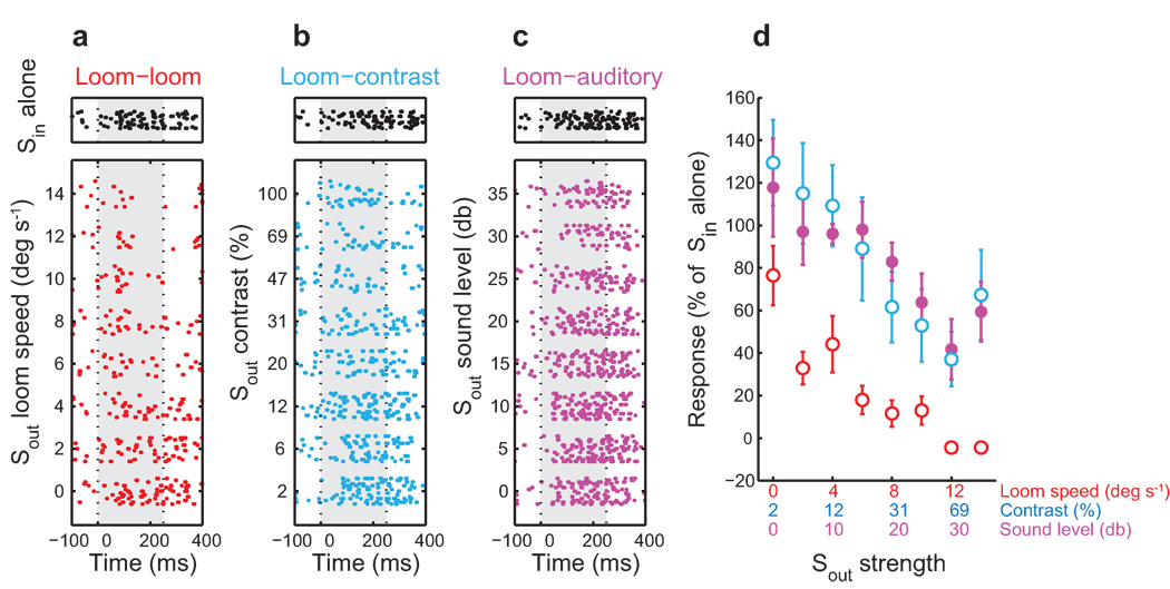
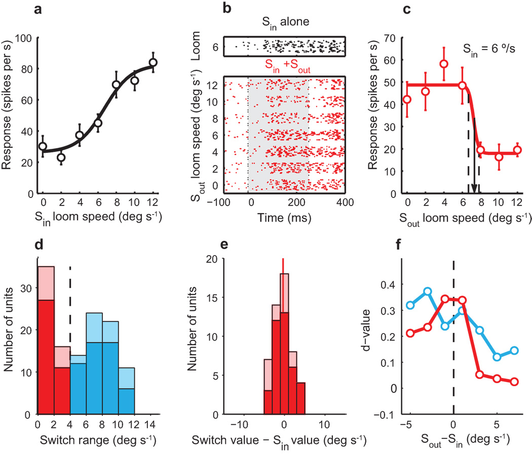
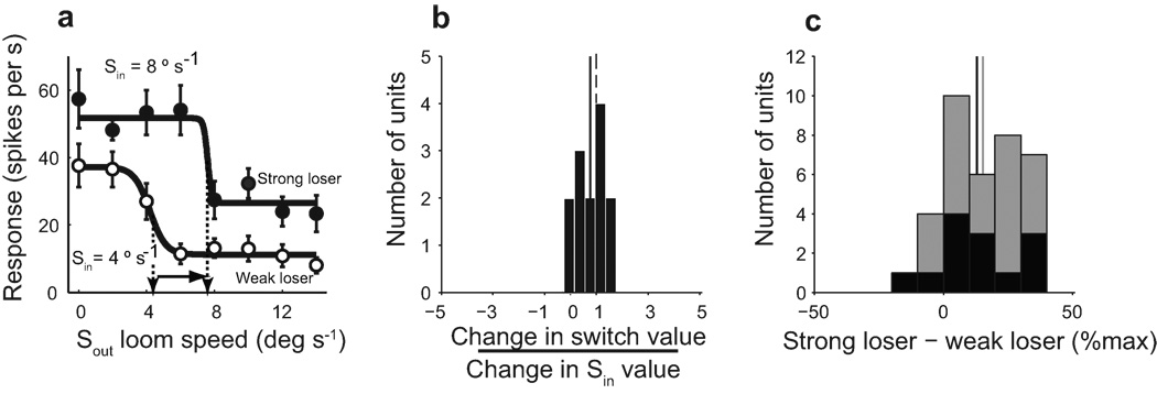
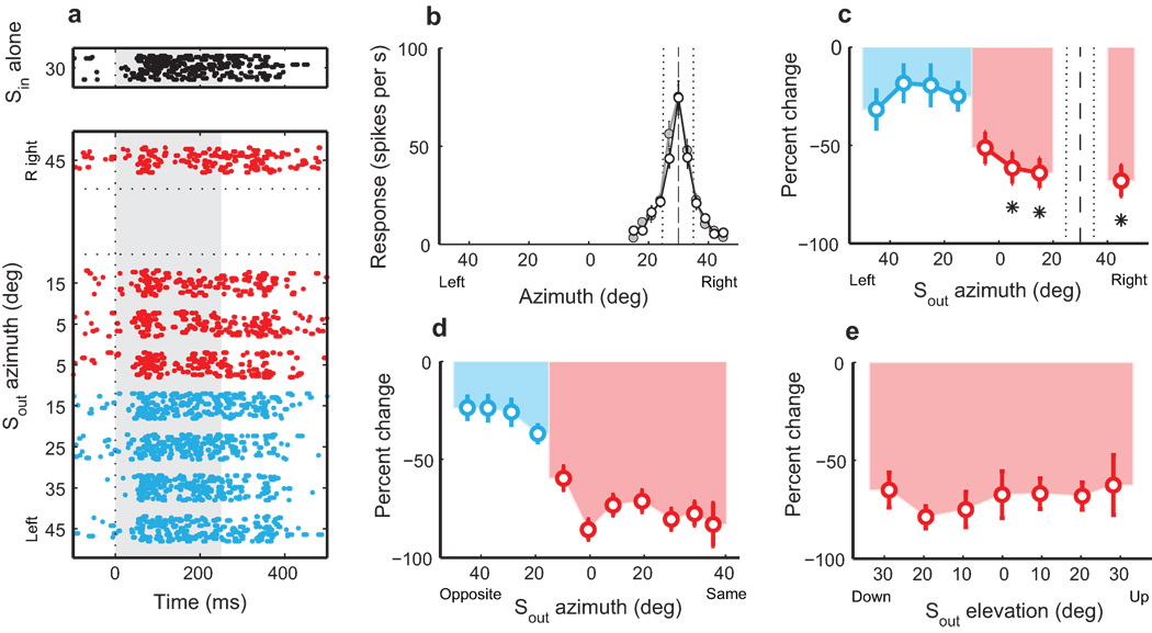
The mechanisms by which the brain selects a particular stimulus as the next target for gaze are poorly understood. A cholinergic nucleus in the owl's midbrain exhibits functional properties that suggest its role in bottom-up stimulus selection. Neurons in the nucleus isthmi pars parvocellularis (Ipc) responded to wide ranges of visual and auditory features, but they were not tuned to particular values of those features. Instead, they encoded the relative strengths of stimuli across the entirety of space. Many neurons exhibited switch-like properties, abruptly increasing their responses to a stimulus in their receptive field when it became the strongest stimulus. This information propagates directly to the optic tectum, a structure involved in gaze control and stimulus selection, as periodic (25-50 Hz) bursts of cholinergic activity. The functional properties of Ipc neurons resembled those of a salience map, a core component in computational models for spatial attention and gaze control.

Figure 1. Feature and modality independence of stimulus competition for a single nonswitch-like Ipc unit

The effect of the strength of a competing stimulus on responses to a dark looming dot (S_in), 80% contrast, 4 °/s, centered in the receptive field at left 11°, +8°. An S_out competitor stimulus was located 30° to the side of the receptive field, at left 41°, +8°. The stimuli were presented simultaneously from 0–250 ms. a) Upper raster: responses to the S_in stimulus presented alone. Lower rasters: responses to the S_in stimulus paired with an 80% contrast, looming dot S_out stimulus with various speeds. b) Responses to the S_in stimulus paired with a looming dot S_out stimulus (speed = 4 °/s) with various contrasts. c) Responses to the S_in stimulus paired with a broadband noise burst S_out stimulus at various sound levels relative to the unit’s threshold. d) Responses to the S_in and S_out stimuli presented together relative to the response to the S_in stimulus alone plotted as a function of S_out strength. Red: S_out = visual loom speed. Blue: S_out = visual loom contrast. Magenta: S_out = auditory noise burst. Responses are normalized by the response to the S_in alone for each profile. All S_out stimuli systematically suppressed the response to the S_in stimulus alone (p<0.05, correlation analysis). Error bars indicate s.e.m.

Figure 2. Effect of a competing looming stimulus on unit responses to a looming stimulus

a) Speed-response function for a single Ipc unit measured with a single looming stimulus centered in the receptive field. Line: sigmoidal fit to the data (Methods). b) Raster representation of the unit’s responses to a looming S_in stimulus (6°/s) presented simultaneously with a looming S_out competitor of different loom speeds. c) The competitor strength-response profile: Mean response values for the responses shown in b. Line: sigmoidal fit to the data (Methods); dashed lines: transition range; arrow: switch value. This unit had a switch-like competitor strength-response profile. d) Distribution of transition ranges for 121 units tested with two looming stimuli; switch-like units (red) and non-switch-like units (blue). The light bars represent data from non-tranquilized owls. e) Distribution of differences between the switch value and the S_in loom speed for all switch-like units. Red line: mean difference = −0.32 ± 0.39 (p=0.3, Wilcoxon signed rank test, n=51). The light bars represent data from non-tranquilized owls. f) Population average d’ values comparing responses to a 2 °/s increment in S_out value, plotted as a function of the average difference between the strengths of S_out and S_in. Red circles: data from switch-like units; blue circles: data from non-switch-like units. Error bars in a and c indicate s.e.m.

Figure 3. Effect of the strength of the S_in stimulus on switch value

a) Competitor strength-response profiles for a switch-like unit measured with two different S_in loom speeds: 4 °/s (open symbols) and 8 °/s (filled symbols). Solid lines: sigmoidal fits to the data; vertical arrows: switch values; horizontal arrow: change in switch value. Error bars indicate s.e.m. b) Ratio of the change in switch value relative to the change in S_in loom speed for switch-like units. All data measured with looming S_in and S_out stimuli. Dashed vertical line: designates one; Solid vertical line: mean ratio for switch units = 0.77; Wilcoxon signed rank test re. 1, n=13, P=0.24. c) The difference between responses to a stronger, “loser” S_in stimulus versus a weaker, “loser” S_in stimulus. Black bars: switch-like units; gray bars: nonswitch-like units. For each unit, the difference is calculated as the average of the responses at S_out= 12 °/s and 14 °/s. The difference is expressed as a percentage of the maximum response to the stronger S_in stimulus presented alone. For switch-like units, an average increase in S_in strength of 4.3 ± 1.2 °/s produced an average response increase of 13 ± 4.7% (Wilcoxon signed rank test re. zero, n=13, P=0.021); for nonswitch-like units, an average increase in S_in strength of 4.5 ± 0.93 °/s produced an average response increase of 15.3 ± 3.5 % (Wilcoxon signed rank test re. zero, n=23, P<0.0001). Black and gray vertical lines represents mean for switch-like and nonswitch-like neurons respectively.

Figure 4. Global stimulus competition in the Ipc

a) Rasters of unit responses to a dark looming (4 °/s) dot stimulus (S_in), centered in the receptive field, with and without a competing, S_out looming stimulus (8 °/s) presented from different azimuths. b) receptive fields of the unit to the S_in (black) and S_out (gray) stimuli presented alone. Dashed line: center of receptive field. Dotted lines: half-max. c) Response of the unit to the S_in and S_out stimuli presented together as a percent of the response to the S_in presented alone. Red circles: mean ± s.e.m. for S_out locations <15° into the hemifield opposite to the receptive field. Blue circles: mean ± s.e.m for S_out locations ≥ 15° into the opposite hemifield. Dashed and dotted lines: receptive field. d,e) Population average suppression of responses to S_in as a function of the location of the S_out stimulus. S_in = 4 or 6 °/s; S_out = 8 or 10 °/s; n=31; mean ± s.e.m. S_out locations more ≥15° from the receptive field center were binned to the nearest 10° increment. d) S_out locations in azimuth. Red and blue circles, as in c. e) S_out locations in elevation.

Figure 5. Periodicity of bursting responses of Ipc units

a) Raster of responses of an Ipc unit to an 8 °/s looming stimulus centered in the receptive field. Dashed lines: response window analyzed for periodicity. b) Multi-taper spectral analysis of the spike pattern shown in a reveals a peak periodicity of 35 Hz. Solid line: mean power spectrum. Dotted lines: jackknife error bars. Dashed line: power spectrum of a hypothetical Poisson spiking neuron with equal firing rate. Deviation from the dashed line represents periodic nature of the phenomenon. c) Distribution of the peaks in the response power spectra for 57 Ipc units. Dashed line: mean ± s.e.m: 36.3 Hz ± 0.7. d) Covariation of average power of spike periodicity, measured in the 20–60 Hz band, and average spike rate for a population of 39 switch-like units, each responding to a looming S_in stimulus presented simultaneously with a looming S_out stimulus of different speeds. The abscissa shows the difference in strength between S_out and S_in. Error bars indicate s.e.m.

References

1. Sommer MA, Wurtz RH. Composition and topographic organization of signals sent from the frontal eye field to the superior colliculus. J Neurophysiol. 2000;83:1979–2001. - PubMed
1. Reynolds JH, Chelazzi L. Attentional modulation of visual processing. Annu Rev Neurosci. 2004;27:611–647. - PubMed
1. McPeek RM, Keller EL. Saccade target selection in the superior colliculus during a visual search task. J Neurophysiol. 2002;88:2019–2034. - PubMed
1. Muller JR, Philiastides MG, Newsome WT. Microstimulation of the superior colliculus focuses attention without moving the eyes. Proc Natl Acad Sci U S A. 2005;102:524–529. - PMC - PubMed
1. Schiller PH, Sandell JH, Maunsell JH. The effect of frontal eye field and superior colliculus lesions on saccadic latencies in the rhesus monkey. J Neurophysiol. 1987;57:1033–1049. - PubMed
Publication types