

Inferring combinatorial association logic networks in multimodal genome-wide screens
- PMID: 20529900
- PMCID: PMC2881395
- DOI: 10.1093/bioinformatics/btq211
Inferring combinatorial association logic networks in multimodal genome-wide screens
Abstract
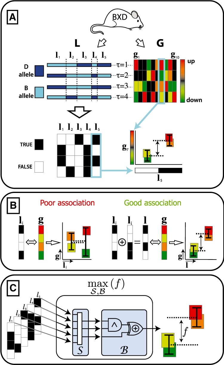
Motivation: We propose an efficient method to infer combinatorial association logic networks from multiple genome-wide measurements from the same sample. We demonstrate our method on a genetical genomics dataset, in which we search for Boolean combinations of multiple genetic loci that associate with transcript levels.
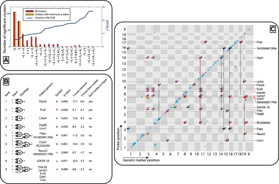
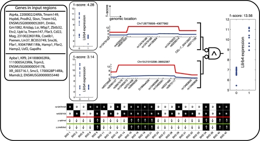
Results: Our method provably finds the global solution and is very efficient with runtimes of up to four orders of magnitude faster than the exhaustive search. This enables permutation procedures for determining accurate false positive rates and allows selection of the most parsimonious model. When applied to transcript levels measured in myeloid cells from 24 genotyped recombinant inbred mouse strains, we discovered that nine gene clusters are putatively modulated by a logical combination of trait loci rather than a single locus. A literature survey supports and further elucidates one of these findings. Due to our approach, optimal solutions for multi-locus logic models and accurate estimates of the associated false discovery rates become feasible. Our algorithm, therefore, offers a valuable alternative to approaches employing complex, albeit suboptimal optimization strategies to identify complex models.
Availability: The MATLAB code of the prototype implementation is available on: http://bioinformatics.tudelft.nl/ or http://bioinformatics.nki.nl/.
Figures
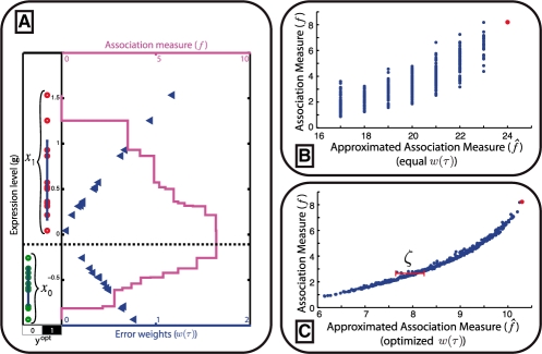
 and f. The red dot indicates
  and f values for yopt. (B) shows the samples in case the weights are assumed equal. Although the trend of the data is monotonically increasing, a large spread around this trend is observed. (C) shows the same samples in case the weights are optimized, resulting in a near one-to-one relation between
  and f.
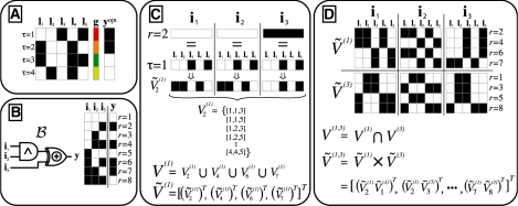
 . To determine the complete set of valid input combinations for τ = 1, rows 4, 6 and 7 need to be considered in a similar fashion. V(1) is now determined by taking the union of the subsets, i.e. V(1) = V2(1)∪V4(1)∪V6(1)∪V7(1), which, in binary form, may be represented by a concatenation of
  ,
,  ,
,  and
and  . (D) This panel shows the valid input combinations for τ = 1 and τ = 3 in binary representation (i.e.
  and
and  ). For any set of samples C the input combinations for which the output equals yopt can be obtained by taking the intersection of the individual sets. In binary representation, this is equivalent to taking the row-wise cartesian product (row-wise product of all combinations of rows), as is shown in the panel.
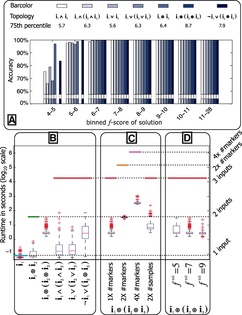
Similar articles
-
MixupMapper: correcting sample mix-ups in genome-wide datasets increases power to detect small genetic effects.Bioinformatics. 2011 Aug 1;27(15):2104-11. doi: 10.1093/bioinformatics/btr323. Epub 2011 Jun 7. Bioinformatics. 2011. PMID: 21653519
-
Simultaneous search for multiple QTL using the global optimization algorithm DIRECT.Bioinformatics. 2004 Aug 12;20(12):1887-95. doi: 10.1093/bioinformatics/bth175. Epub 2004 Mar 25. Bioinformatics. 2004. PMID: 15044246
-
An effective framework for reconstructing gene regulatory networks from genetical genomics data.Bioinformatics. 2013 Jan 15;29(2):246-54. doi: 10.1093/bioinformatics/bts679. Epub 2012 Nov 21. Bioinformatics. 2013. PMID: 23175757
-
Inferring gene transcriptional modulatory relations: a genetical genomics approach.Hum Mol Genet. 2005 May 1;14(9):1119-25. doi: 10.1093/hmg/ddi124. Epub 2005 Mar 16. Hum Mol Genet. 2005. PMID: 15772094
-
Review of microarray experimental design strategies for genetical genomics studies.Physiol Genomics. 2006 Dec 13;28(1):15-23. doi: 10.1152/physiolgenomics.00106.2006. Epub 2006 Sep 19. Physiol Genomics. 2006. PMID: 16985008 Review.
Cited by
-
Logic models to predict continuous outputs based on binary inputs with an application to personalized cancer therapy.Sci Rep. 2016 Nov 23;6:36812. doi: 10.1038/srep36812. Sci Rep. 2016. PMID: 27876821 Free PMC article.
-
High-throughput semiquantitative analysis of insertional mutations in heterogeneous tumors.Genome Res. 2011 Dec;21(12):2181-9. doi: 10.1101/gr.112763.110. Epub 2011 Aug 18. Genome Res. 2011. PMID: 21852388 Free PMC article.
References
-
- Bystrykh LV, et al. Uncovering regulatory pathways that affect hematopoietic stem cell function using ‘genetical genomics’. Nat. Genet. 2005;37:225–232. - PubMed
-
- Castells MC, et al. gp49b1-alpha(v)beta3 interaction inhibits antigen-induced mast cell activation. Nat. Immunol. 2001;2:436–442. - PubMed
-
- Cleveland W. Robust locally weighted regression and smoothing scatterplots. J. Am. Stat. Assoc. 1979;74:829–836.
