

Validation of coevolving residue algorithms via pipeline sensitivity analysis: ELSC and OMES and ZNMI, oh my!
- PMID: 20531955
- PMCID: PMC2879359
- DOI: 10.1371/journal.pone.0010779
Validation of coevolving residue algorithms via pipeline sensitivity analysis: ELSC and OMES and ZNMI, oh my!
Abstract
Correlated amino acid substitution algorithms attempt to discover groups of residues that co-fluctuate due to either structural or functional constraints. Although these algorithms could inform both ab initio protein folding calculations and evolutionary studies, their utility for these purposes has been hindered by a lack of confidence in their predictions due to hard to control sources of error. To complicate matters further, naive users are confronted with a multitude of methods to choose from, in addition to the mechanics of assembling and pruning a dataset. We first introduce a new pair scoring method, called ZNMI (Z-scored-product Normalized Mutual Information), which drastically improves the performance of mutual information for co-fluctuating residue prediction. Second and more important, we recast the process of finding coevolving residues in proteins as a data-processing pipeline inspired by the medical imaging literature. We construct an ensemble of alignment partitions that can be used in a cross-validation scheme to assess the effects of choices made during the procedure on the resulting predictions. This pipeline sensitivity study gives a measure of reproducibility (how similar are the predictions given perturbations to the pipeline?) and accuracy (are residue pairs with large couplings on average close in tertiary structure?). We choose a handful of published methods, along with ZNMI, and compare their reproducibility and accuracy on three diverse protein families. We find that (i) of the algorithms tested, while none appear to be both highly reproducible and accurate, ZNMI is one of the most accurate by far and (ii) while users should be wary of predictions drawn from a single alignment, considering an ensemble of sub-alignments can help to determine both highly accurate and reproducible couplings. Our cross-validation approach should be of interest both to developers and end users of algorithms that try to detect correlated amino acid substitutions.
Conflict of interest statement
Figures
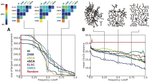
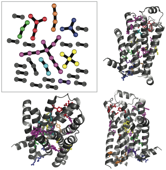
 distance. Directly above the plot, the consensus graph is shown at three different edge frequency cutoffs. Note the dramatic transition in the consensus graph between a weight of 0.25 and 0.5; simply removing edges which co-occur less than 50% of the time results in a network consisting primary of small, disjoint clusters. Notice also that even at a cutoff of 0.75, many nontrivial clusters (beyond simple pairs) remain in the network.
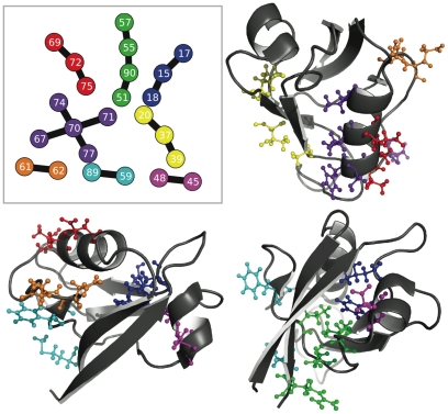
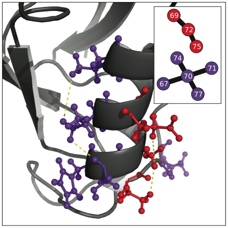
 -helix.
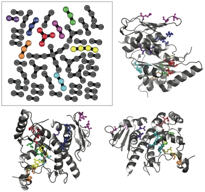
References
-
- Martin L, Gloor G, Dunn S, Wahl L. Using information theory to search for co-evolving residues in proteins. Bioinformatics. 2005;21:4116–4124. - PubMed
-
- Atchley WR, Wollenberg KR, Fitch WM, Terhalle W, Dress AW. Correlations among amino acid sites in bhlh protein domains: an information theoretic analysis. Molecular Biology and Evolution. 2000;17:164–178. - PubMed
-
- Horner D, Pirovano W, Pesole G. Correlated substitution analysis and the prediction of amino acid structural contacts. Briefings in Bioinformatics. 2007;9:46–56. - PubMed
-
- Ashkenazy H, Unger R, Kliger Y. Optimal data collection for correlated mutation analysis. Proteins. 2009;74:545–555. - PubMed
Publication types
MeSH terms
Substances
LinkOut - more resources
Full Text Sources
