Principal semantic components of language and the measurement of meaning

Abstract

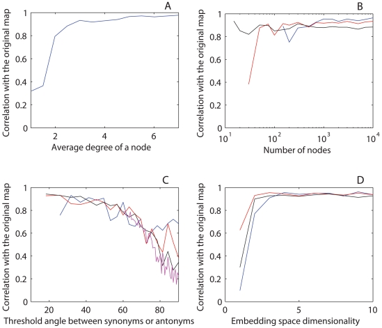
Metric systems for semantics, or semantic cognitive maps, are allocations of words or other representations in a metric space based on their meaning. Existing methods for semantic mapping, such as Latent Semantic Analysis and Latent Dirichlet Allocation, are based on paradigms involving dissimilarity metrics. They typically do not take into account relations of antonymy and yield a large number of domain-specific semantic dimensions. Here, using a novel self-organization approach, we construct a low-dimensional, context-independent semantic map of natural language that represents simultaneously synonymy and antonymy. Emergent semantics of the map principal components are clearly identifiable: the first three correspond to the meanings of "good/bad" (valence), "calm/excited" (arousal), and "open/closed" (freedom), respectively. The semantic map is sufficiently robust to allow the automated extraction of synonyms and antonyms not originally in the dictionaries used to construct the map and to predict connotation from their coordinates. The map geometric characteristics include a limited number ( approximately 4) of statistically significant dimensions, a bimodal distribution of the first component, increasing kurtosis of subsequent (unimodal) components, and a U-shaped maximum-spread planar projection. Both the semantic content and the main geometric features of the map are consistent between dictionaries (Microsoft Word and Princeton's WordNet), among Western languages (English, French, German, and Spanish), and with previously established psychometric measures. By defining the semantics of its dimensions, the constructed map provides a foundational metric system for the quantitative analysis of word meaning. Language can be viewed as a cumulative product of human experiences. Therefore, the extracted principal semantic dimensions may be useful to characterize the general semantic dimensions of the content of mental states. This is a fundamental step toward a universal metric system for semantics of human experiences, which is necessary for developing a rigorous science of the mind.

Figure 1. Principal components (PCs) of the constructed semantic map.

Distributions of words in maximal-spread projections (PC2 vs. PC1) are shown in panels A–C. Coordinates are normalized by the squared-average vector length of all words. A: MS (Microsoft Word) English, B: WN (WordNet 3.0) English, C: MS French. D: MS English in PC3–PC4 coordinates. Representative words are labeled and identical terms or automated word-to-word translations are marked by same colors on different panels. The small blue dots represent all words of the corpora. A small random subset of words is plotted in light blue to aid visibility of individual dots in the face of excessive density (e.g., in panel C). Similarity of relative word positions is evident across panels A–C, but not D.

Figure 2. Standard deviations and kurtosis of the first PCs in the MS English map.

Inset: distributions of word projections onto the first 3 PCs normalized to unit area under the curve.

Figure 3. Semantic map correspondence across languages and methodologies.

The scatter plots demonstrate numerical correspondence between MS English PC1 and both WN English PC1 (blue) and the first ANEW dimension, ‘pleasure’ (red). The dashed line represents the common linear fit. Captions show correlation coefficients (R), corresponding P-values, and numbers N of common words used for the analysis. All three distributions (MS English PC1, WN English PC1, and ANEW pleasure) are clearly bimodal. The correlations are highly significant even when analyzed for the two separate clusters of data. For words with negative MS English PC1 values, the correlation with the corresponding WN English PC1 values is R = 0.46 (p<10⁻¹⁰, N = 3101); and with ANEW: R = 0.36 (p<10⁻⁷, N = 226). For the positive MS English values, R = 0.40 for WN English (p<10⁻¹⁰, N = 2825) and R = 0.39 for ANEW (p<10⁻⁸, N = 225).

Figure 4. Values of the first four PCs for four different words in the MS English semantic map.

PC coordinate values are represented in the bars, while the corresponding numbers express these quantities as percentages of the standard deviation of each PC (cf. Figure 2).

Figure 5. Angular distributions of word pairs on the map.

The plots represent histograms of angle distributions for synonyms (1, blue), antonyms (2, red), onyms of onyms not listed as onyms (3, solid black line), and unrelated words (4, dashed line). Here “onym” stands for “synonym or antonym”, and onyms of onyms include synonyms of synonyms, synonyms of antonyms, antonyms of synonyms, and antonyms of antonyms.

Figure 6. Semantics of the cognitive map (MS English): examples of connotation mapping.

For each of the two representative (bold and circled) words, control and delicate, 8 synonyms are selected such that they nearly uniformly occupy all quadrants.

Figure 7. Semantic characteristics of the frequency of word usage.

A: cumulative distribution of vector length of all words in MS English, with dotted horizontal lines at the 2.5^th, 50^th, and 97.5^th percentiles. The arrow indicates the mean weighted by the British National Corpus (BNC) frequency distribution. B: MS English word sorting by the frequency of their usage according to two independent sources (see Materials and Methods): Australian database (blue) and BNC (red). C: Values of the first 4 PCs of the weighted average of all words according to the Australian database frequencies. As in Figure 4, the bars and corresponding numbers represent the PC coordinate values and their percentage of the standard deviation of each PC (in the case of BNC frequencies, the corresponding numbers are: 64.0+7.5%, 13.3+6.4%, −15.4+11.9%, and 10.2+6.4%). Standard errors are reported for both bars (as whiskers) and numbers. Only the first component is statistically significant.

Figure 8. Reconstruction of the color map.

A: original PC standard deviations in d = 10. B: standard deviations of PCs in the starting configuration selected for optimization. C: reconstructed PC standard deviations in d = 10. D: original color space map. E: reconstructed color space map.

Figure 9. Robustness of the color map reconstruction.

A: correlation between the reconstructed map and the original map as it varies with the embedding space dimension d for three different values of the threshold angle between “onyms”: 10° (blue), 20° (red), and 30° (black). The number of nodes and their average degree are 1000 and 3.5, respectively. B: correlation between the reconstructed and the original map as a function of the average node degree. The number of nodes, embedding dimension, and threshold value are 1000, 10, and 0.90, respectively. C: correlation with the original map as a function of the number of nodes. The embedding dimension, threshold, and average degree are 10, 0.50, and 3.5, respectively. D: correlation with the original map as a function of the threshold angle between “synonyms” and “antonyms” for four different values of the number of nodes: 100 (blue), 300 (red), 1000 (black), 5000 (magenta). The embedding dimension and average degree are 10 and 3.50, respectively.

Figure 10. Semantic space concept.

X: space of concepts (meanings) internally delineated by distinct domains of applicability; V: space of relations among concepts; G: graph of relations among selected concepts in X. Links connecting concepts in X and in G are translated to common origin in V and rotated to minimize the energy function (*), while preserving their consistent angular relations that correspond to the notions of synonymy and antonymy.

References

-
- Fellbaum C. WordNet: An electronic lexical database. Cambridge, MA: MIT Press; 1998.
- Ascoli GA, Samsonovich AV. Science of the conscious mind. Biol Bull. 2008;215:204–215. - PubMed
- Tversky A, Gati I. Similarity, separability, and the triangle inequality. Psychol Rev. 1982;89:123–154. - PubMed
- Landauer TK, Dumais ST. A solution to Plato's problem: the Latent Semantic Analysis theory of acquisition, induction, and representation of knowledge. Psyc Rev. 1997;104:211–240.
- Landauer TK, McNamara DS, Dennis S, Kintsch W, editors. Handbook of Latent Semantic Analysis. Mahwah, NJ: Lawrence Erlbaum Associates; 2007.
Publication types
MeSH terms
LinkOut - more resources
Full Text Sources
Other Literature Sources
Research Materials