Fast nonnegative deconvolution for spike train inference from population calcium imaging

Abstract

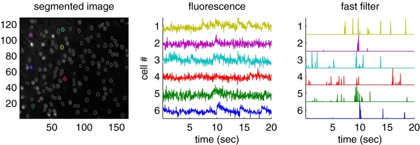
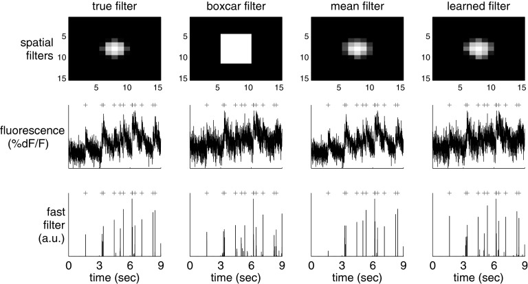
Fluorescent calcium indicators are becoming increasingly popular as a means for observing the spiking activity of large neuronal populations. Unfortunately, extracting the spike train of each neuron from a raw fluorescence movie is a nontrivial problem. This work presents a fast nonnegative deconvolution filter to infer the approximately most likely spike train of each neuron, given the fluorescence observations. This algorithm outperforms optimal linear deconvolution (Wiener filtering) on both simulated and biological data. The performance gains come from restricting the inferred spike trains to be positive (using an interior-point method), unlike the Wiener filter. The algorithm runs in linear time, and is fast enough that even when simultaneously imaging >100 neurons, inference can be performed on the set of all observed traces faster than real time. Performing optimal spatial filtering on the images further refines the inferred spike train estimates. Importantly, all the parameters required to perform the inference can be estimated using only the fluorescence data, obviating the need to perform joint electrophysiological and imaging calibration experiments.

Fig. 1.

Typical in vitro data suggest that a reasonable first-order model may be constructed by convolving the spike train with an exponential and adding Gaussian noise. Top panel: the average (over frames) of a field of view. Bottom left: true spike train recorded via a patch electrode (black bars), convolved with an exponential (gray line), superimposed on the Oregon Green BAPTA 1 (OGB-1) fluorescence trace (black line). Whereas the spike train and fluorescence trace are measured data, the calcium is not directly measured, but rather, inferred. Bottom right: a histogram of the residual error between the gray and black lines from the bottom left panel (dashed line) and the best-fit Gaussian (solid line). Note that the Gaussian model provides a good fit for the residuals here.

Fig. 2.

A simulation showing that the fast filter's inferred spike train is significantly more accurate than the output of the optimal linear deconvolution (Wiener filter). Note that neither filter constrains the inference to be a sequence of integers; rather, the fast filter relaxes the constraint to allow all nonnegative numbers and the Wiener filter allows for all real numbers. The restriction of the fast filter to exclude negative numbers eliminates the ringing effect seen in the Wiener filter output, resulting in a much cleaner inference. Note that the magnitude of the inferred spikes in the fast filter output is proportional to the inferred calcium jump size. Top panel: fluorescence trace. Second panel: spike train. Third panel: fast filter inference. Bottom panel: Wiener filter inference. Note that the gray bars in the bottom panel indicate negative spikes. Gray + symbols indicate true spike times. Simulation details: T = 400 time steps, Δ = 33.3 ms, α = 1, β = 0, σ = 0.2, τ = 1 s, λ = 1 Hz. Parameters and conventions are consistent across figures, unless indicated otherwise.

Fig. 3.

In simulations, the fast filter quantitatively and significantly achieves higher accuracy than that of the Wiener filter. Top left: a spike train (bottom) and 2 simulated fluorescence traces, using the same spike train, one with low signal-to-noise ratio (SNR) (middle) and one with high SNR (top). Simulation parameters: τ = 0.5 s, λ = 3 Hz, Δ = 1/30 s, σ = 0.6 (low SNR) and 0.1 (high SNR). Simulation parameters in other panels are the same, except where explicitly noted. Top right: mean-squared-error (MSE) for the fast (solid line) and Wiener (dashed-dotted line) filter, for varying the expected firing rate λ. Note that both axes are on a log-scale. Further note that the fast filter has a better (lower) MSE for all expected firing rates. Error bars show SD over 10 repeats. Simulation parameters: σ = 0.2, T = 1,000 time steps. Bottom left: receiver-operator-characteristic (ROC) curve comparing the fast (solid line) and Wiener (dashed-dotted line) filter. Note that for any given threshold, the Wiener filter has a better (higher) ratio of true positive rate to false positive rate. Simulation parameters as in top right panel, except σ = 0.35 and T = 10,000 time steps. Bottom right: area under the curve (AUC) for fast (solid line) and Wiener (dashed-dotted line) filter as a function of SD (σ). Note that the fast filter has a better (higher) AUC for all σ values until noise gets very high. The 2 simulated fluorescence traces in the top left panel show the bounds for SD here. Error bars show SD over 10 repeats.

Fig. 4.

A simulation showing that the fast filter achieves significantly more accurate inference than that of the Wiener filter, even when the parameters are unknown. For both filters, the appropriate parameters were estimated using only the data shown above, unlike Fig. 2, in which the true parameters were provided to the filters. Simulation details different from those in Fig. 2: T = 1,000 time steps, Δ = 16.7 ms, σ = 0.4.

Fig. 5.

In vitro data showing that the fast filter significantly outperforms the Wiener filter, using OGB-1. Note that all the parameters for both filters were estimated only from the fluorescence data in the top panel (i.e., not considering the voltage data at all). + symbols denote true spike times extracted from the patch data, not inferred spike times from F.

Fig. 6.

In vitro data with multispike events, showing that the fast filter can often resolve the correct number of spikes within each spiking event, while imaging using OGB-1, given sufficiently high SNR. It is difficult, if not impossible, to count the number of spikes given the Wiener filter output. Recording and fitting parameters as in Fig. 5. Note that the parameters were estimated using a 60-s-long recording, of which only a fraction is shown here, to more clearly depict the number of spikes per event.

Fig. 7.

The fast filter infers spike trains from a large population of neurons imaged simultaneously in vitro, faster than real time. Specifically, inferring the spike trains from this 400-s-long movie including 136 neurons required only about 40 s on a standard laptop computer. The inferred spike trains much more clearly convey neural activity than the raw fluorescence traces. Although no intracellular “ground truth” is available from these population data, the noise seems to be reduced, consistent with the other examples with ground truth. Left: mean image field, automatically segmented into regions of interest (ROIs), each containing a single neuron using custom software. Middle: example fluorescence traces. Right: fast filter output corresponding to each associated trace. Note that neuron identity is indicated by color across the 3 panels. Data were collected using a confocal microscope and Fura-2, as described in methods.

Fig. 8.

In vitro data with SNR of only about 3 (estimated by dividing the fluorescent jump size by the SD of the baseline fluorescence) for single action potentials depicting the fast filter, effectively initializing the parameters for the sequential Monte Carlo (SMC) filter, significantly reducing the number of expectation-maximization iterations to convergence, using OGB-1. Note that whereas the fast filter clearly infers the spiking events in the end of the trace, those in the beginning of the trace are less clear. On the other hand, the SMC filter more clearly separates nonspiking activity from true spikes. Also note that the ordinate on the third panel corresponds to the inferred probability of a spike having occurred in each frame.

Fig. 9.

A simulation demonstrating that using a better spatial filter can significantly enhance the effective SNR. The true spatial filter was a difference of Gaussians: a positively weighted Gaussian of small width and a negatively weighted Gaussian with larger width (both with the same center). Each column shows the spatial filter (top), one-dimensional fluorescence projection using that spatial filter (middle), and inferred spike train (bottom). From left to right, columns use the true, boxcar, mean, and learned spatial filter obtained using Eq. 29. Note that the learned filter's inferred spike train has fewer false positives and negatives than the boxcar and mean filters. 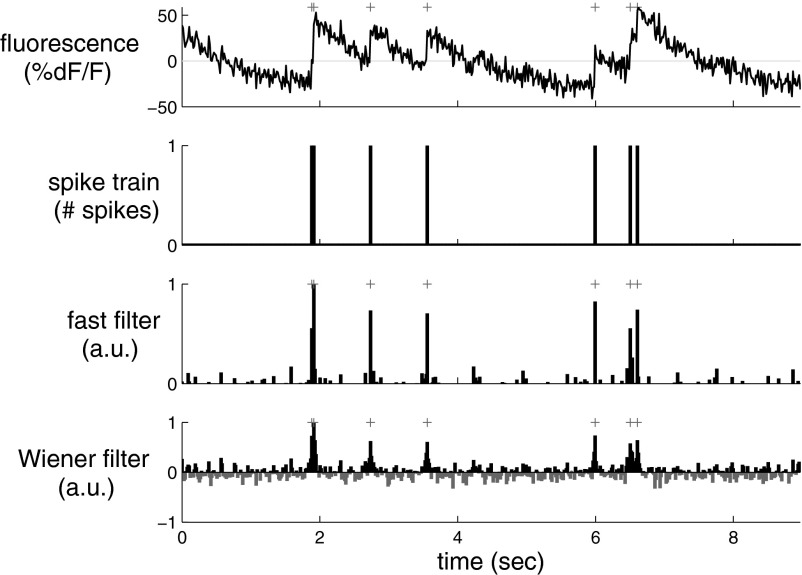Simulation parameters: α→ = (0, 2I) − 0.5(0, 2.5I), where (μ, Σ) indicates a 2-dimensional Gaussian with mean μ and covariance matrix Σ, β→ = 0, σ = 0.2, τ = 0.85 s, λ = 5 Hz, Δ = 5 ms, T = 1,200 time steps.

Fig. 10.

Simulation showing that when 2 neurons' spatial filters are largely overlapping, learning the optimal spatial filters using Eq. 36 can yield improved inference of the standard boxcar type filters. The 3 columns show the effect of the true (left), boxcar (center), and learned (right) spatial filters. A: the sum of the 2 spatial filters for each approach, clearly depicting overlap. B: the spatial filters (top row), one-dimensional fluorescence projection, and inferred spike train (bottom row) for one of the neurons. C: same as B for the other neuron. Note that the inferred spike trains when using the learned filter are close to optimal, unlike the boxcar filter. Simulation parameters: α→¹ = ([−1, 0], 2I) − 0.5([−1, 0], 2.5I), α→² = ([1, 0], 2I) − 0.5([1, 0], 2.5I), β→ = 0, σ = 0.02, τ = 0.5 s, λ = 5 Hz, Δ = 5 ms, T = 1,200 time steps (not all time steps are shown).

References

-
- Andrieu C, Barat É, Doucet A. Bayesian deconvolution of noisy filtered point processes. IEEE Trans Signal Process 49: 134–146, 2001
- Bell AJ, Sejnowski TJ. An information-maximisation approach to blind separation and blind deconvolution. Neural Comput 7: 1129–1159, 1995 - PubMed
- Boyd S, Vandenberghe L. Convex Optimization. Cambridge, UK: Cambridge Univ. Press, 2004
- Cover TM, Thomas JA. Elements of Information Theory: New York: Wiley–Interscience, 1991
- Cunningham JP, Shenoy KV, Sahani M. Fast Gaussian process methods for point process intensity estimation. In: Proceedings of the 25th International Conference on Machine Learning (ICML 2008) New York: IEEE Press, 2008, p. 192–199
Publication types
MeSH terms
Substances
Grants and funding
LinkOut - more resources
Full Text Sources
Other Literature Sources