

Review
doi: 10.1016/j.clinph.2010.04.037.
Epub 2010 Jun 22.
Subdural electrodes
Affiliations
- PMID: 20573543
- PMCID: PMC2962988
- DOI: 10.1016/j.clinph.2010.04.037
Item in Clipboard
Review
Subdural electrodes
Clin Neurophysiol.
2010 Sep.
Abstract
Subdural electrodes are frequently used to aid in the neurophysiological assessment of patients with intractable seizures. We review the indications for these, their uses for localizing epileptogenic regions and for localizing cortical regions supporting movement, sensation, and language.
2010 International Federation of Clinical Neurophysiology. Published by Elsevier Ireland Ltd. All rights reserved.
Figures
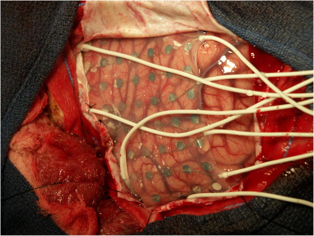
Subdural electrode placements can vary with the individual. In this patient a large array is present in the center of the figure. On the left of the figure are two “pigtail” wires that come from two subdural strips anterior to the grid. At the bottom are two pigtails from subdural arrays placed below to temporal lobe. Left is anterior, right posterior, cortex. The vertex is superior and basal hemisphere regions inferior. Electrode centers are separated by 1 cm.
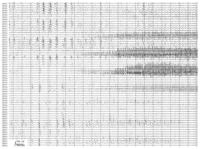
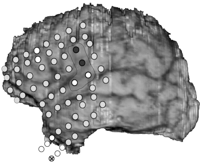
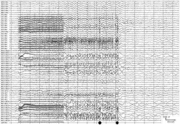
Two seizure onsets from two different cortical sites. Fig. 2a shows a seizure originating from the left rolandic region, electrodes LFT23, 31 (filled circles, Fig. 2c) with reflection at and spread to adjacent electrodes. Fig. 2b shows a seizure originating from the left anterior temporal lobe, LBT57, again with spread to adjacent electrodes. Recording was at 200 samples/second and used a 0.5 Hz high pass and 70 Hz low pass filter; the filters were single pole RC filters with 6db/octave rolloff. Fig. 2c shows electrode locations. A 64 electrode grid was in place, with the top 6 rows over the lateral, primarily suprasylvian, cortex and the bottom two rows over the temporal lobe, directed towards, and with the anterior three electrodes in each row wrapped around, the temporal tip. The grid was cut between row 6 and 7 to facilitate placement. Numbering goes from 1 at the upper left, to 8 at the upper right, to 48 at the lower right of the superior six rows (LFT in Fig. 2a and 2b). Numbering for the inferior 2 rows (LBT) goes from 57 for the anterior electrode in the top row to 64 for the posterior electrode in the bottom row. Electrodes LFT 23 and 31 are filled, and electrode LBT57 has an X through it. The “boot” around electrodes LFT 23 and 31 plus two other electrodes indicates where stimulation mapping found motor cortex. Recording display is to a system reference. The patient was 15 years old, with a history of meningoencephalitis 5 years earlier. Seizures began with arousal from sleep and head deviation to the right.
Two seizure onsets from two different cortical sites. Fig. 2a shows a seizure originating from the left rolandic region, electrodes LFT23, 31 (filled circles, Fig. 2c) with reflection at and spread to adjacent electrodes. Fig. 2b shows a seizure originating from the left anterior temporal lobe, LBT57, again with spread to adjacent electrodes. Recording was at 200 samples/second and used a 0.5 Hz high pass and 70 Hz low pass filter; the filters were single pole RC filters with 6db/octave rolloff. Fig. 2c shows electrode locations. A 64 electrode grid was in place, with the top 6 rows over the lateral, primarily suprasylvian, cortex and the bottom two rows over the temporal lobe, directed towards, and with the anterior three electrodes in each row wrapped around, the temporal tip. The grid was cut between row 6 and 7 to facilitate placement. Numbering goes from 1 at the upper left, to 8 at the upper right, to 48 at the lower right of the superior six rows (LFT in Fig. 2a and 2b). Numbering for the inferior 2 rows (LBT) goes from 57 for the anterior electrode in the top row to 64 for the posterior electrode in the bottom row. Electrodes LFT 23 and 31 are filled, and electrode LBT57 has an X through it. The “boot” around electrodes LFT 23 and 31 plus two other electrodes indicates where stimulation mapping found motor cortex. Recording display is to a system reference. The patient was 15 years old, with a history of meningoencephalitis 5 years earlier. Seizures began with arousal from sleep and head deviation to the right.
Two seizure onsets from two different cortical sites. Fig. 2a shows a seizure originating from the left rolandic region, electrodes LFT23, 31 (filled circles, Fig. 2c) with reflection at and spread to adjacent electrodes. Fig. 2b shows a seizure originating from the left anterior temporal lobe, LBT57, again with spread to adjacent electrodes. Recording was at 200 samples/second and used a 0.5 Hz high pass and 70 Hz low pass filter; the filters were single pole RC filters with 6db/octave rolloff. Fig. 2c shows electrode locations. A 64 electrode grid was in place, with the top 6 rows over the lateral, primarily suprasylvian, cortex and the bottom two rows over the temporal lobe, directed towards, and with the anterior three electrodes in each row wrapped around, the temporal tip. The grid was cut between row 6 and 7 to facilitate placement. Numbering goes from 1 at the upper left, to 8 at the upper right, to 48 at the lower right of the superior six rows (LFT in Fig. 2a and 2b). Numbering for the inferior 2 rows (LBT) goes from 57 for the anterior electrode in the top row to 64 for the posterior electrode in the bottom row. Electrodes LFT 23 and 31 are filled, and electrode LBT57 has an X through it. The “boot” around electrodes LFT 23 and 31 plus two other electrodes indicates where stimulation mapping found motor cortex. Recording display is to a system reference. The patient was 15 years old, with a history of meningoencephalitis 5 years earlier. Seizures began with arousal from sleep and head deviation to the right.
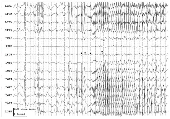
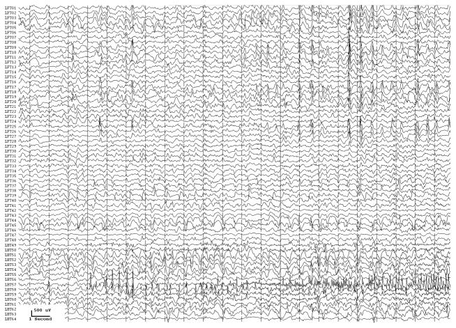
Figure 3a shows onset of a seizure from the left anterior frontal lobe. In recordings from this region there were almost constant interictal bursts from LFP1-5 and LOF3-8. The first two dots between the EEG channels from LFP7 and LFP8 occur at the same time as the last interictal discharges before a spontaneous seizure starts. Seizure onset is just before the time of the third dot, particularly at electrodes LFP1-5 and LOF 3-8, and manifested by much faster activity than occurred during the interictal discharges. Voltage appears to decrease at LFP7-8, between the times of dots 3 and 4. We use the four dots to help in orienting between figures; they indicate the same points in time in each of the figures in which they appear. Recording was at 1000 samples/second and used a 0.5 Hz high pass and 300 Hz low pass filter. The filters were second order Butterworth with 12 db/Oct rolloff. Figure 3b shows a time expansion of a portion of the recording in Fig. 3a. In addition to the fast activity just described, there is still faster activity at LFP7-8, where there appeared to be voltage decrement before. This is best seen when voltage is increased. (Compare channels 6 and 8 - showing the EEG at the same amplification as in the other channels - versus channels 7 and 9 - showing the EEG at higher amplification.) Figure 3c shows electrode placement. The numbering for electrodes in each strip is 1–8. Electrode 1 is the most inferior electrode for RLF-RFP-LFP, the most mesial electrode for LOF, and the most anterior electrode for LAT. For LFG, 1 is the most anterior and 8 the most posterior electrode on the top row; the most anterior and posterior electrode for the fifth row are 33 and 40 respectively. The 64 electrode grid was cut between rows 5 and 6, and the most anterior electrode for row 6 is 41, the most anterior electrode for row 8 is 57, and the most posterior electrode for row 8 is 64. In this patient, electrode LOF1 was used as the ground; LFP4 was not functioning properly. Recording display is to a system reference. Seizures persisted after resection of the region showing conventional epileptiform activity in Fig. 3A. The patient became seizure free after a second resection 18 months later, that was posterior to the first, and included LFP7-8 and LOF8. Figures 3d and 3e are visualizations of the contributions of higher frequencies to the EEG in this instance. Fig. 3d shows 70–200 Hz and Fig. 3e 214-300 Hz activity. There is a gap between 200 and 214 Hz to avoid frequency overlap. Activity in the 70–200 Hz frequency range begins about 200 msec before the third dot in a number of channels, particularly LFP1-3, LOF7-8. Some activity in the 214-300 Hz range appears at LFP2 at the same time, but this becomes widespread at about the time of the third dot and in particular is at LFP7-8 and LOF8, lasting about 3 seconds. These figures use an enhanced display method to preserves the amplitude of the high frequency information at conventional time resolutions. First we use a high pass digital filter to suppress low frequency signals. This then sets the bandwidth of our high frequency observation. Next for each successive group of ten samples we note the maximum and minimum values. The display process then draws a vertical between each maximum and minimum pair for each group of ten original data points. Thus the range of amplitudes is preserved even as the data rate for the data stream is reduced. Other methods of display at standard time resolutions can in effect filter out this information. For example, typical computer screens can only manage 100 pixels per second of data when displaying EEG traces conventional resolutions analogous to 30 mm/second for paper EEG. This is due to the pixel size of the display monitor. When sampling the original EEG at 1000 sample/second, the display can only show one data point in ten. In effect this down samples the EEG by a factor of ten because of the screen display rate. Any data above the Nyquist frequency (i.e. half sample rate) of the screen display rate is lost or distorted. Typically there are two other display methods used to reduce high sample rate data for display. Decimation uses only one sample in 10 and results in aliasing of frequency components above Nyquist frequency. Averaging of successive groups of 10 samples produces a data stream of one tenth the sample rate and effectively filters out any high frequency components. Neither method is ideal for showing the amplitude of any high frequency information present in the EEG. Fig. 3f shows activity at LFP8. EEG activity is at the top. The bottom uses a color display to show that activity in different frequency ranges appears and disappears at different times during the recording. The Y axis indicates frequency using a logarithmic scale. The X axis indicates elapsed time in seconds. The colors indicate amplitude in log microvolt units, as shown at the bottom. Fig. 3g and Fig. 3h show progressively more channels of the recording, with fig. 3h showing all the recorded channels. The patient was 39 years old, with seizures since age 20; there was no known cause. Seizures began with anxiety, tingling in the shoulders and loss of ability to interact appropriately. An MRI had shown possible increased T2 signal in, and decreased size of, left mesial temporal structures. PET scan had shown bilateral hypometabolism sparing an area in the left temporal lobe at a time with frequent seizures, and mildly reduced fluorodeoxyglucose uptake in the left mesial temporal region in a second study 19 months later, but before the first grid placement and frontal resection. Seizure onset did not include the mesial temporal lobe, temporal lobe was not removed, and the patient became seizure free after the second frontal resection.
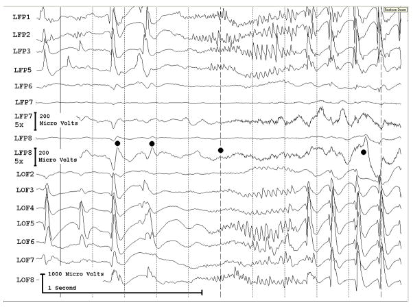
Figure 3a shows onset of a seizure from the left anterior frontal lobe. In recordings from this region there were almost constant interictal bursts from LFP1-5 and LOF3-8. The first two dots between the EEG channels from LFP7 and LFP8 occur at the same time as the last interictal discharges before a spontaneous seizure starts. Seizure onset is just before the time of the third dot, particularly at electrodes LFP1-5 and LOF 3-8, and manifested by much faster activity than occurred during the interictal discharges. Voltage appears to decrease at LFP7-8, between the times of dots 3 and 4. We use the four dots to help in orienting between figures; they indicate the same points in time in each of the figures in which they appear. Recording was at 1000 samples/second and used a 0.5 Hz high pass and 300 Hz low pass filter. The filters were second order Butterworth with 12 db/Oct rolloff. Figure 3b shows a time expansion of a portion of the recording in Fig. 3a. In addition to the fast activity just described, there is still faster activity at LFP7-8, where there appeared to be voltage decrement before. This is best seen when voltage is increased. (Compare channels 6 and 8 - showing the EEG at the same amplification as in the other channels - versus channels 7 and 9 - showing the EEG at higher amplification.) Figure 3c shows electrode placement. The numbering for electrodes in each strip is 1–8. Electrode 1 is the most inferior electrode for RLF-RFP-LFP, the most mesial electrode for LOF, and the most anterior electrode for LAT. For LFG, 1 is the most anterior and 8 the most posterior electrode on the top row; the most anterior and posterior electrode for the fifth row are 33 and 40 respectively. The 64 electrode grid was cut between rows 5 and 6, and the most anterior electrode for row 6 is 41, the most anterior electrode for row 8 is 57, and the most posterior electrode for row 8 is 64. In this patient, electrode LOF1 was used as the ground; LFP4 was not functioning properly. Recording display is to a system reference. Seizures persisted after resection of the region showing conventional epileptiform activity in Fig. 3A. The patient became seizure free after a second resection 18 months later, that was posterior to the first, and included LFP7-8 and LOF8. Figures 3d and 3e are visualizations of the contributions of higher frequencies to the EEG in this instance. Fig. 3d shows 70–200 Hz and Fig. 3e 214-300 Hz activity. There is a gap between 200 and 214 Hz to avoid frequency overlap. Activity in the 70–200 Hz frequency range begins about 200 msec before the third dot in a number of channels, particularly LFP1-3, LOF7-8. Some activity in the 214-300 Hz range appears at LFP2 at the same time, but this becomes widespread at about the time of the third dot and in particular is at LFP7-8 and LOF8, lasting about 3 seconds. These figures use an enhanced display method to preserves the amplitude of the high frequency information at conventional time resolutions. First we use a high pass digital filter to suppress low frequency signals. This then sets the bandwidth of our high frequency observation. Next for each successive group of ten samples we note the maximum and minimum values. The display process then draws a vertical between each maximum and minimum pair for each group of ten original data points. Thus the range of amplitudes is preserved even as the data rate for the data stream is reduced. Other methods of display at standard time resolutions can in effect filter out this information. For example, typical computer screens can only manage 100 pixels per second of data when displaying EEG traces conventional resolutions analogous to 30 mm/second for paper EEG. This is due to the pixel size of the display monitor. When sampling the original EEG at 1000 sample/second, the display can only show one data point in ten. In effect this down samples the EEG by a factor of ten because of the screen display rate. Any data above the Nyquist frequency (i.e. half sample rate) of the screen display rate is lost or distorted. Typically there are two other display methods used to reduce high sample rate data for display. Decimation uses only one sample in 10 and results in aliasing of frequency components above Nyquist frequency. Averaging of successive groups of 10 samples produces a data stream of one tenth the sample rate and effectively filters out any high frequency components. Neither method is ideal for showing the amplitude of any high frequency information present in the EEG. Fig. 3f shows activity at LFP8. EEG activity is at the top. The bottom uses a color display to show that activity in different frequency ranges appears and disappears at different times during the recording. The Y axis indicates frequency using a logarithmic scale. The X axis indicates elapsed time in seconds. The colors indicate amplitude in log microvolt units, as shown at the bottom. Fig. 3g and Fig. 3h show progressively more channels of the recording, with fig. 3h showing all the recorded channels. The patient was 39 years old, with seizures since age 20; there was no known cause. Seizures began with anxiety, tingling in the shoulders and loss of ability to interact appropriately. An MRI had shown possible increased T2 signal in, and decreased size of, left mesial temporal structures. PET scan had shown bilateral hypometabolism sparing an area in the left temporal lobe at a time with frequent seizures, and mildly reduced fluorodeoxyglucose uptake in the left mesial temporal region in a second study 19 months later, but before the first grid placement and frontal resection. Seizure onset did not include the mesial temporal lobe, temporal lobe was not removed, and the patient became seizure free after the second frontal resection.
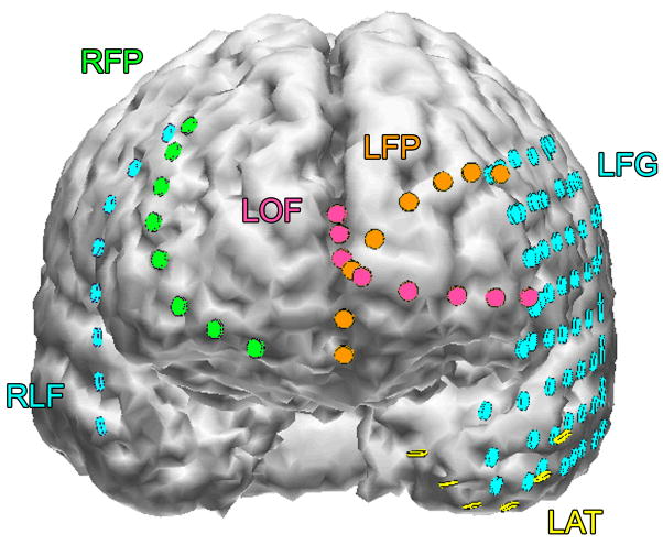
Figure 3a shows onset of a seizure from the left anterior frontal lobe. In recordings from this region there were almost constant interictal bursts from LFP1-5 and LOF3-8. The first two dots between the EEG channels from LFP7 and LFP8 occur at the same time as the last interictal discharges before a spontaneous seizure starts. Seizure onset is just before the time of the third dot, particularly at electrodes LFP1-5 and LOF 3-8, and manifested by much faster activity than occurred during the interictal discharges. Voltage appears to decrease at LFP7-8, between the times of dots 3 and 4. We use the four dots to help in orienting between figures; they indicate the same points in time in each of the figures in which they appear. Recording was at 1000 samples/second and used a 0.5 Hz high pass and 300 Hz low pass filter. The filters were second order Butterworth with 12 db/Oct rolloff. Figure 3b shows a time expansion of a portion of the recording in Fig. 3a. In addition to the fast activity just described, there is still faster activity at LFP7-8, where there appeared to be voltage decrement before. This is best seen when voltage is increased. (Compare channels 6 and 8 - showing the EEG at the same amplification as in the other channels - versus channels 7 and 9 - showing the EEG at higher amplification.) Figure 3c shows electrode placement. The numbering for electrodes in each strip is 1–8. Electrode 1 is the most inferior electrode for RLF-RFP-LFP, the most mesial electrode for LOF, and the most anterior electrode for LAT. For LFG, 1 is the most anterior and 8 the most posterior electrode on the top row; the most anterior and posterior electrode for the fifth row are 33 and 40 respectively. The 64 electrode grid was cut between rows 5 and 6, and the most anterior electrode for row 6 is 41, the most anterior electrode for row 8 is 57, and the most posterior electrode for row 8 is 64. In this patient, electrode LOF1 was used as the ground; LFP4 was not functioning properly. Recording display is to a system reference. Seizures persisted after resection of the region showing conventional epileptiform activity in Fig. 3A. The patient became seizure free after a second resection 18 months later, that was posterior to the first, and included LFP7-8 and LOF8. Figures 3d and 3e are visualizations of the contributions of higher frequencies to the EEG in this instance. Fig. 3d shows 70–200 Hz and Fig. 3e 214-300 Hz activity. There is a gap between 200 and 214 Hz to avoid frequency overlap. Activity in the 70–200 Hz frequency range begins about 200 msec before the third dot in a number of channels, particularly LFP1-3, LOF7-8. Some activity in the 214-300 Hz range appears at LFP2 at the same time, but this becomes widespread at about the time of the third dot and in particular is at LFP7-8 and LOF8, lasting about 3 seconds. These figures use an enhanced display method to preserves the amplitude of the high frequency information at conventional time resolutions. First we use a high pass digital filter to suppress low frequency signals. This then sets the bandwidth of our high frequency observation. Next for each successive group of ten samples we note the maximum and minimum values. The display process then draws a vertical between each maximum and minimum pair for each group of ten original data points. Thus the range of amplitudes is preserved even as the data rate for the data stream is reduced. Other methods of display at standard time resolutions can in effect filter out this information. For example, typical computer screens can only manage 100 pixels per second of data when displaying EEG traces conventional resolutions analogous to 30 mm/second for paper EEG. This is due to the pixel size of the display monitor. When sampling the original EEG at 1000 sample/second, the display can only show one data point in ten. In effect this down samples the EEG by a factor of ten because of the screen display rate. Any data above the Nyquist frequency (i.e. half sample rate) of the screen display rate is lost or distorted. Typically there are two other display methods used to reduce high sample rate data for display. Decimation uses only one sample in 10 and results in aliasing of frequency components above Nyquist frequency. Averaging of successive groups of 10 samples produces a data stream of one tenth the sample rate and effectively filters out any high frequency components. Neither method is ideal for showing the amplitude of any high frequency information present in the EEG. Fig. 3f shows activity at LFP8. EEG activity is at the top. The bottom uses a color display to show that activity in different frequency ranges appears and disappears at different times during the recording. The Y axis indicates frequency using a logarithmic scale. The X axis indicates elapsed time in seconds. The colors indicate amplitude in log microvolt units, as shown at the bottom. Fig. 3g and Fig. 3h show progressively more channels of the recording, with fig. 3h showing all the recorded channels. The patient was 39 years old, with seizures since age 20; there was no known cause. Seizures began with anxiety, tingling in the shoulders and loss of ability to interact appropriately. An MRI had shown possible increased T2 signal in, and decreased size of, left mesial temporal structures. PET scan had shown bilateral hypometabolism sparing an area in the left temporal lobe at a time with frequent seizures, and mildly reduced fluorodeoxyglucose uptake in the left mesial temporal region in a second study 19 months later, but before the first grid placement and frontal resection. Seizure onset did not include the mesial temporal lobe, temporal lobe was not removed, and the patient became seizure free after the second frontal resection.
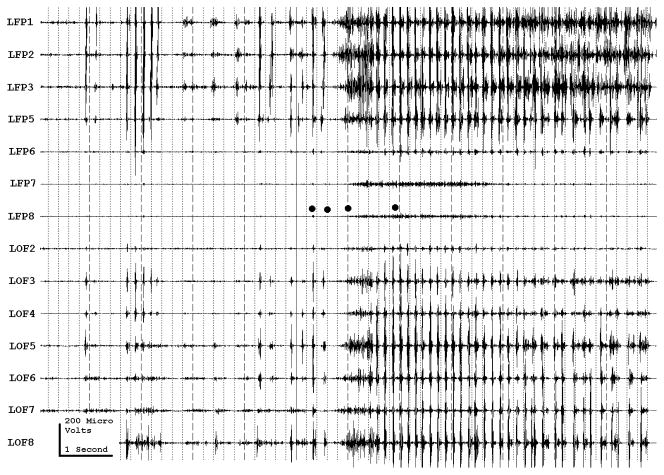
Figure 3a shows onset of a seizure from the left anterior frontal lobe. In recordings from this region there were almost constant interictal bursts from LFP1-5 and LOF3-8. The first two dots between the EEG channels from LFP7 and LFP8 occur at the same time as the last interictal discharges before a spontaneous seizure starts. Seizure onset is just before the time of the third dot, particularly at electrodes LFP1-5 and LOF 3-8, and manifested by much faster activity than occurred during the interictal discharges. Voltage appears to decrease at LFP7-8, between the times of dots 3 and 4. We use the four dots to help in orienting between figures; they indicate the same points in time in each of the figures in which they appear. Recording was at 1000 samples/second and used a 0.5 Hz high pass and 300 Hz low pass filter. The filters were second order Butterworth with 12 db/Oct rolloff. Figure 3b shows a time expansion of a portion of the recording in Fig. 3a. In addition to the fast activity just described, there is still faster activity at LFP7-8, where there appeared to be voltage decrement before. This is best seen when voltage is increased. (Compare channels 6 and 8 - showing the EEG at the same amplification as in the other channels - versus channels 7 and 9 - showing the EEG at higher amplification.) Figure 3c shows electrode placement. The numbering for electrodes in each strip is 1–8. Electrode 1 is the most inferior electrode for RLF-RFP-LFP, the most mesial electrode for LOF, and the most anterior electrode for LAT. For LFG, 1 is the most anterior and 8 the most posterior electrode on the top row; the most anterior and posterior electrode for the fifth row are 33 and 40 respectively. The 64 electrode grid was cut between rows 5 and 6, and the most anterior electrode for row 6 is 41, the most anterior electrode for row 8 is 57, and the most posterior electrode for row 8 is 64. In this patient, electrode LOF1 was used as the ground; LFP4 was not functioning properly. Recording display is to a system reference. Seizures persisted after resection of the region showing conventional epileptiform activity in Fig. 3A. The patient became seizure free after a second resection 18 months later, that was posterior to the first, and included LFP7-8 and LOF8. Figures 3d and 3e are visualizations of the contributions of higher frequencies to the EEG in this instance. Fig. 3d shows 70–200 Hz and Fig. 3e 214-300 Hz activity. There is a gap between 200 and 214 Hz to avoid frequency overlap. Activity in the 70–200 Hz frequency range begins about 200 msec before the third dot in a number of channels, particularly LFP1-3, LOF7-8. Some activity in the 214-300 Hz range appears at LFP2 at the same time, but this becomes widespread at about the time of the third dot and in particular is at LFP7-8 and LOF8, lasting about 3 seconds. These figures use an enhanced display method to preserves the amplitude of the high frequency information at conventional time resolutions. First we use a high pass digital filter to suppress low frequency signals. This then sets the bandwidth of our high frequency observation. Next for each successive group of ten samples we note the maximum and minimum values. The display process then draws a vertical between each maximum and minimum pair for each group of ten original data points. Thus the range of amplitudes is preserved even as the data rate for the data stream is reduced. Other methods of display at standard time resolutions can in effect filter out this information. For example, typical computer screens can only manage 100 pixels per second of data when displaying EEG traces conventional resolutions analogous to 30 mm/second for paper EEG. This is due to the pixel size of the display monitor. When sampling the original EEG at 1000 sample/second, the display can only show one data point in ten. In effect this down samples the EEG by a factor of ten because of the screen display rate. Any data above the Nyquist frequency (i.e. half sample rate) of the screen display rate is lost or distorted. Typically there are two other display methods used to reduce high sample rate data for display. Decimation uses only one sample in 10 and results in aliasing of frequency components above Nyquist frequency. Averaging of successive groups of 10 samples produces a data stream of one tenth the sample rate and effectively filters out any high frequency components. Neither method is ideal for showing the amplitude of any high frequency information present in the EEG. Fig. 3f shows activity at LFP8. EEG activity is at the top. The bottom uses a color display to show that activity in different frequency ranges appears and disappears at different times during the recording. The Y axis indicates frequency using a logarithmic scale. The X axis indicates elapsed time in seconds. The colors indicate amplitude in log microvolt units, as shown at the bottom. Fig. 3g and Fig. 3h show progressively more channels of the recording, with fig. 3h showing all the recorded channels. The patient was 39 years old, with seizures since age 20; there was no known cause. Seizures began with anxiety, tingling in the shoulders and loss of ability to interact appropriately. An MRI had shown possible increased T2 signal in, and decreased size of, left mesial temporal structures. PET scan had shown bilateral hypometabolism sparing an area in the left temporal lobe at a time with frequent seizures, and mildly reduced fluorodeoxyglucose uptake in the left mesial temporal region in a second study 19 months later, but before the first grid placement and frontal resection. Seizure onset did not include the mesial temporal lobe, temporal lobe was not removed, and the patient became seizure free after the second frontal resection.
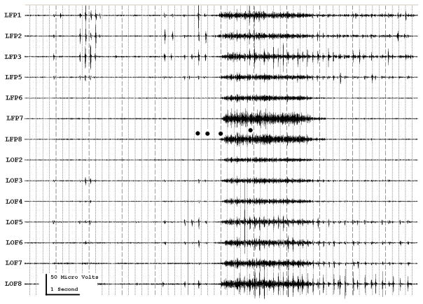
Figure 3a shows onset of a seizure from the left anterior frontal lobe. In recordings from this region there were almost constant interictal bursts from LFP1-5 and LOF3-8. The first two dots between the EEG channels from LFP7 and LFP8 occur at the same time as the last interictal discharges before a spontaneous seizure starts. Seizure onset is just before the time of the third dot, particularly at electrodes LFP1-5 and LOF 3-8, and manifested by much faster activity than occurred during the interictal discharges. Voltage appears to decrease at LFP7-8, between the times of dots 3 and 4. We use the four dots to help in orienting between figures; they indicate the same points in time in each of the figures in which they appear. Recording was at 1000 samples/second and used a 0.5 Hz high pass and 300 Hz low pass filter. The filters were second order Butterworth with 12 db/Oct rolloff. Figure 3b shows a time expansion of a portion of the recording in Fig. 3a. In addition to the fast activity just described, there is still faster activity at LFP7-8, where there appeared to be voltage decrement before. This is best seen when voltage is increased. (Compare channels 6 and 8 - showing the EEG at the same amplification as in the other channels - versus channels 7 and 9 - showing the EEG at higher amplification.) Figure 3c shows electrode placement. The numbering for electrodes in each strip is 1–8. Electrode 1 is the most inferior electrode for RLF-RFP-LFP, the most mesial electrode for LOF, and the most anterior electrode for LAT. For LFG, 1 is the most anterior and 8 the most posterior electrode on the top row; the most anterior and posterior electrode for the fifth row are 33 and 40 respectively. The 64 electrode grid was cut between rows 5 and 6, and the most anterior electrode for row 6 is 41, the most anterior electrode for row 8 is 57, and the most posterior electrode for row 8 is 64. In this patient, electrode LOF1 was used as the ground; LFP4 was not functioning properly. Recording display is to a system reference. Seizures persisted after resection of the region showing conventional epileptiform activity in Fig. 3A. The patient became seizure free after a second resection 18 months later, that was posterior to the first, and included LFP7-8 and LOF8. Figures 3d and 3e are visualizations of the contributions of higher frequencies to the EEG in this instance. Fig. 3d shows 70–200 Hz and Fig. 3e 214-300 Hz activity. There is a gap between 200 and 214 Hz to avoid frequency overlap. Activity in the 70–200 Hz frequency range begins about 200 msec before the third dot in a number of channels, particularly LFP1-3, LOF7-8. Some activity in the 214-300 Hz range appears at LFP2 at the same time, but this becomes widespread at about the time of the third dot and in particular is at LFP7-8 and LOF8, lasting about 3 seconds. These figures use an enhanced display method to preserves the amplitude of the high frequency information at conventional time resolutions. First we use a high pass digital filter to suppress low frequency signals. This then sets the bandwidth of our high frequency observation. Next for each successive group of ten samples we note the maximum and minimum values. The display process then draws a vertical between each maximum and minimum pair for each group of ten original data points. Thus the range of amplitudes is preserved even as the data rate for the data stream is reduced. Other methods of display at standard time resolutions can in effect filter out this information. For example, typical computer screens can only manage 100 pixels per second of data when displaying EEG traces conventional resolutions analogous to 30 mm/second for paper EEG. This is due to the pixel size of the display monitor. When sampling the original EEG at 1000 sample/second, the display can only show one data point in ten. In effect this down samples the EEG by a factor of ten because of the screen display rate. Any data above the Nyquist frequency (i.e. half sample rate) of the screen display rate is lost or distorted. Typically there are two other display methods used to reduce high sample rate data for display. Decimation uses only one sample in 10 and results in aliasing of frequency components above Nyquist frequency. Averaging of successive groups of 10 samples produces a data stream of one tenth the sample rate and effectively filters out any high frequency components. Neither method is ideal for showing the amplitude of any high frequency information present in the EEG. Fig. 3f shows activity at LFP8. EEG activity is at the top. The bottom uses a color display to show that activity in different frequency ranges appears and disappears at different times during the recording. The Y axis indicates frequency using a logarithmic scale. The X axis indicates elapsed time in seconds. The colors indicate amplitude in log microvolt units, as shown at the bottom. Fig. 3g and Fig. 3h show progressively more channels of the recording, with fig. 3h showing all the recorded channels. The patient was 39 years old, with seizures since age 20; there was no known cause. Seizures began with anxiety, tingling in the shoulders and loss of ability to interact appropriately. An MRI had shown possible increased T2 signal in, and decreased size of, left mesial temporal structures. PET scan had shown bilateral hypometabolism sparing an area in the left temporal lobe at a time with frequent seizures, and mildly reduced fluorodeoxyglucose uptake in the left mesial temporal region in a second study 19 months later, but before the first grid placement and frontal resection. Seizure onset did not include the mesial temporal lobe, temporal lobe was not removed, and the patient became seizure free after the second frontal resection.
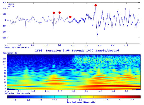
Figure 3a shows onset of a seizure from the left anterior frontal lobe. In recordings from this region there were almost constant interictal bursts from LFP1-5 and LOF3-8. The first two dots between the EEG channels from LFP7 and LFP8 occur at the same time as the last interictal discharges before a spontaneous seizure starts. Seizure onset is just before the time of the third dot, particularly at electrodes LFP1-5 and LOF 3-8, and manifested by much faster activity than occurred during the interictal discharges. Voltage appears to decrease at LFP7-8, between the times of dots 3 and 4. We use the four dots to help in orienting between figures; they indicate the same points in time in each of the figures in which they appear. Recording was at 1000 samples/second and used a 0.5 Hz high pass and 300 Hz low pass filter. The filters were second order Butterworth with 12 db/Oct rolloff. Figure 3b shows a time expansion of a portion of the recording in Fig. 3a. In addition to the fast activity just described, there is still faster activity at LFP7-8, where there appeared to be voltage decrement before. This is best seen when voltage is increased. (Compare channels 6 and 8 - showing the EEG at the same amplification as in the other channels - versus channels 7 and 9 - showing the EEG at higher amplification.) Figure 3c shows electrode placement. The numbering for electrodes in each strip is 1–8. Electrode 1 is the most inferior electrode for RLF-RFP-LFP, the most mesial electrode for LOF, and the most anterior electrode for LAT. For LFG, 1 is the most anterior and 8 the most posterior electrode on the top row; the most anterior and posterior electrode for the fifth row are 33 and 40 respectively. The 64 electrode grid was cut between rows 5 and 6, and the most anterior electrode for row 6 is 41, the most anterior electrode for row 8 is 57, and the most posterior electrode for row 8 is 64. In this patient, electrode LOF1 was used as the ground; LFP4 was not functioning properly. Recording display is to a system reference. Seizures persisted after resection of the region showing conventional epileptiform activity in Fig. 3A. The patient became seizure free after a second resection 18 months later, that was posterior to the first, and included LFP7-8 and LOF8. Figures 3d and 3e are visualizations of the contributions of higher frequencies to the EEG in this instance. Fig. 3d shows 70–200 Hz and Fig. 3e 214-300 Hz activity. There is a gap between 200 and 214 Hz to avoid frequency overlap. Activity in the 70–200 Hz frequency range begins about 200 msec before the third dot in a number of channels, particularly LFP1-3, LOF7-8. Some activity in the 214-300 Hz range appears at LFP2 at the same time, but this becomes widespread at about the time of the third dot and in particular is at LFP7-8 and LOF8, lasting about 3 seconds. These figures use an enhanced display method to preserves the amplitude of the high frequency information at conventional time resolutions. First we use a high pass digital filter to suppress low frequency signals. This then sets the bandwidth of our high frequency observation. Next for each successive group of ten samples we note the maximum and minimum values. The display process then draws a vertical between each maximum and minimum pair for each group of ten original data points. Thus the range of amplitudes is preserved even as the data rate for the data stream is reduced. Other methods of display at standard time resolutions can in effect filter out this information. For example, typical computer screens can only manage 100 pixels per second of data when displaying EEG traces conventional resolutions analogous to 30 mm/second for paper EEG. This is due to the pixel size of the display monitor. When sampling the original EEG at 1000 sample/second, the display can only show one data point in ten. In effect this down samples the EEG by a factor of ten because of the screen display rate. Any data above the Nyquist frequency (i.e. half sample rate) of the screen display rate is lost or distorted. Typically there are two other display methods used to reduce high sample rate data for display. Decimation uses only one sample in 10 and results in aliasing of frequency components above Nyquist frequency. Averaging of successive groups of 10 samples produces a data stream of one tenth the sample rate and effectively filters out any high frequency components. Neither method is ideal for showing the amplitude of any high frequency information present in the EEG. Fig. 3f shows activity at LFP8. EEG activity is at the top. The bottom uses a color display to show that activity in different frequency ranges appears and disappears at different times during the recording. The Y axis indicates frequency using a logarithmic scale. The X axis indicates elapsed time in seconds. The colors indicate amplitude in log microvolt units, as shown at the bottom. Fig. 3g and Fig. 3h show progressively more channels of the recording, with fig. 3h showing all the recorded channels. The patient was 39 years old, with seizures since age 20; there was no known cause. Seizures began with anxiety, tingling in the shoulders and loss of ability to interact appropriately. An MRI had shown possible increased T2 signal in, and decreased size of, left mesial temporal structures. PET scan had shown bilateral hypometabolism sparing an area in the left temporal lobe at a time with frequent seizures, and mildly reduced fluorodeoxyglucose uptake in the left mesial temporal region in a second study 19 months later, but before the first grid placement and frontal resection. Seizure onset did not include the mesial temporal lobe, temporal lobe was not removed, and the patient became seizure free after the second frontal resection.
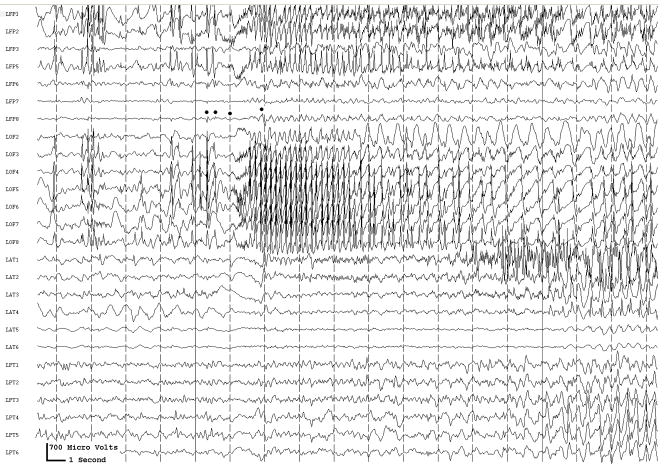
Figure 3a shows onset of a seizure from the left anterior frontal lobe. In recordings from this region there were almost constant interictal bursts from LFP1-5 and LOF3-8. The first two dots between the EEG channels from LFP7 and LFP8 occur at the same time as the last interictal discharges before a spontaneous seizure starts. Seizure onset is just before the time of the third dot, particularly at electrodes LFP1-5 and LOF 3-8, and manifested by much faster activity than occurred during the interictal discharges. Voltage appears to decrease at LFP7-8, between the times of dots 3 and 4. We use the four dots to help in orienting between figures; they indicate the same points in time in each of the figures in which they appear. Recording was at 1000 samples/second and used a 0.5 Hz high pass and 300 Hz low pass filter. The filters were second order Butterworth with 12 db/Oct rolloff. Figure 3b shows a time expansion of a portion of the recording in Fig. 3a. In addition to the fast activity just described, there is still faster activity at LFP7-8, where there appeared to be voltage decrement before. This is best seen when voltage is increased. (Compare channels 6 and 8 - showing the EEG at the same amplification as in the other channels - versus channels 7 and 9 - showing the EEG at higher amplification.) Figure 3c shows electrode placement. The numbering for electrodes in each strip is 1–8. Electrode 1 is the most inferior electrode for RLF-RFP-LFP, the most mesial electrode for LOF, and the most anterior electrode for LAT. For LFG, 1 is the most anterior and 8 the most posterior electrode on the top row; the most anterior and posterior electrode for the fifth row are 33 and 40 respectively. The 64 electrode grid was cut between rows 5 and 6, and the most anterior electrode for row 6 is 41, the most anterior electrode for row 8 is 57, and the most posterior electrode for row 8 is 64. In this patient, electrode LOF1 was used as the ground; LFP4 was not functioning properly. Recording display is to a system reference. Seizures persisted after resection of the region showing conventional epileptiform activity in Fig. 3A. The patient became seizure free after a second resection 18 months later, that was posterior to the first, and included LFP7-8 and LOF8. Figures 3d and 3e are visualizations of the contributions of higher frequencies to the EEG in this instance. Fig. 3d shows 70–200 Hz and Fig. 3e 214-300 Hz activity. There is a gap between 200 and 214 Hz to avoid frequency overlap. Activity in the 70–200 Hz frequency range begins about 200 msec before the third dot in a number of channels, particularly LFP1-3, LOF7-8. Some activity in the 214-300 Hz range appears at LFP2 at the same time, but this becomes widespread at about the time of the third dot and in particular is at LFP7-8 and LOF8, lasting about 3 seconds. These figures use an enhanced display method to preserves the amplitude of the high frequency information at conventional time resolutions. First we use a high pass digital filter to suppress low frequency signals. This then sets the bandwidth of our high frequency observation. Next for each successive group of ten samples we note the maximum and minimum values. The display process then draws a vertical between each maximum and minimum pair for each group of ten original data points. Thus the range of amplitudes is preserved even as the data rate for the data stream is reduced. Other methods of display at standard time resolutions can in effect filter out this information. For example, typical computer screens can only manage 100 pixels per second of data when displaying EEG traces conventional resolutions analogous to 30 mm/second for paper EEG. This is due to the pixel size of the display monitor. When sampling the original EEG at 1000 sample/second, the display can only show one data point in ten. In effect this down samples the EEG by a factor of ten because of the screen display rate. Any data above the Nyquist frequency (i.e. half sample rate) of the screen display rate is lost or distorted. Typically there are two other display methods used to reduce high sample rate data for display. Decimation uses only one sample in 10 and results in aliasing of frequency components above Nyquist frequency. Averaging of successive groups of 10 samples produces a data stream of one tenth the sample rate and effectively filters out any high frequency components. Neither method is ideal for showing the amplitude of any high frequency information present in the EEG. Fig. 3f shows activity at LFP8. EEG activity is at the top. The bottom uses a color display to show that activity in different frequency ranges appears and disappears at different times during the recording. The Y axis indicates frequency using a logarithmic scale. The X axis indicates elapsed time in seconds. The colors indicate amplitude in log microvolt units, as shown at the bottom. Fig. 3g and Fig. 3h show progressively more channels of the recording, with fig. 3h showing all the recorded channels. The patient was 39 years old, with seizures since age 20; there was no known cause. Seizures began with anxiety, tingling in the shoulders and loss of ability to interact appropriately. An MRI had shown possible increased T2 signal in, and decreased size of, left mesial temporal structures. PET scan had shown bilateral hypometabolism sparing an area in the left temporal lobe at a time with frequent seizures, and mildly reduced fluorodeoxyglucose uptake in the left mesial temporal region in a second study 19 months later, but before the first grid placement and frontal resection. Seizure onset did not include the mesial temporal lobe, temporal lobe was not removed, and the patient became seizure free after the second frontal resection.
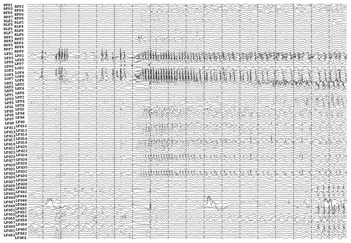
Figure 3a shows onset of a seizure from the left anterior frontal lobe. In recordings from this region there were almost constant interictal bursts from LFP1-5 and LOF3-8. The first two dots between the EEG channels from LFP7 and LFP8 occur at the same time as the last interictal discharges before a spontaneous seizure starts. Seizure onset is just before the time of the third dot, particularly at electrodes LFP1-5 and LOF 3-8, and manifested by much faster activity than occurred during the interictal discharges. Voltage appears to decrease at LFP7-8, between the times of dots 3 and 4. We use the four dots to help in orienting between figures; they indicate the same points in time in each of the figures in which they appear. Recording was at 1000 samples/second and used a 0.5 Hz high pass and 300 Hz low pass filter. The filters were second order Butterworth with 12 db/Oct rolloff. Figure 3b shows a time expansion of a portion of the recording in Fig. 3a. In addition to the fast activity just described, there is still faster activity at LFP7-8, where there appeared to be voltage decrement before. This is best seen when voltage is increased. (Compare channels 6 and 8 - showing the EEG at the same amplification as in the other channels - versus channels 7 and 9 - showing the EEG at higher amplification.) Figure 3c shows electrode placement. The numbering for electrodes in each strip is 1–8. Electrode 1 is the most inferior electrode for RLF-RFP-LFP, the most mesial electrode for LOF, and the most anterior electrode for LAT. For LFG, 1 is the most anterior and 8 the most posterior electrode on the top row; the most anterior and posterior electrode for the fifth row are 33 and 40 respectively. The 64 electrode grid was cut between rows 5 and 6, and the most anterior electrode for row 6 is 41, the most anterior electrode for row 8 is 57, and the most posterior electrode for row 8 is 64. In this patient, electrode LOF1 was used as the ground; LFP4 was not functioning properly. Recording display is to a system reference. Seizures persisted after resection of the region showing conventional epileptiform activity in Fig. 3A. The patient became seizure free after a second resection 18 months later, that was posterior to the first, and included LFP7-8 and LOF8. Figures 3d and 3e are visualizations of the contributions of higher frequencies to the EEG in this instance. Fig. 3d shows 70–200 Hz and Fig. 3e 214-300 Hz activity. There is a gap between 200 and 214 Hz to avoid frequency overlap. Activity in the 70–200 Hz frequency range begins about 200 msec before the third dot in a number of channels, particularly LFP1-3, LOF7-8. Some activity in the 214-300 Hz range appears at LFP2 at the same time, but this becomes widespread at about the time of the third dot and in particular is at LFP7-8 and LOF8, lasting about 3 seconds. These figures use an enhanced display method to preserves the amplitude of the high frequency information at conventional time resolutions. First we use a high pass digital filter to suppress low frequency signals. This then sets the bandwidth of our high frequency observation. Next for each successive group of ten samples we note the maximum and minimum values. The display process then draws a vertical between each maximum and minimum pair for each group of ten original data points. Thus the range of amplitudes is preserved even as the data rate for the data stream is reduced. Other methods of display at standard time resolutions can in effect filter out this information. For example, typical computer screens can only manage 100 pixels per second of data when displaying EEG traces conventional resolutions analogous to 30 mm/second for paper EEG. This is due to the pixel size of the display monitor. When sampling the original EEG at 1000 sample/second, the display can only show one data point in ten. In effect this down samples the EEG by a factor of ten because of the screen display rate. Any data above the Nyquist frequency (i.e. half sample rate) of the screen display rate is lost or distorted. Typically there are two other display methods used to reduce high sample rate data for display. Decimation uses only one sample in 10 and results in aliasing of frequency components above Nyquist frequency. Averaging of successive groups of 10 samples produces a data stream of one tenth the sample rate and effectively filters out any high frequency components. Neither method is ideal for showing the amplitude of any high frequency information present in the EEG. Fig. 3f shows activity at LFP8. EEG activity is at the top. The bottom uses a color display to show that activity in different frequency ranges appears and disappears at different times during the recording. The Y axis indicates frequency using a logarithmic scale. The X axis indicates elapsed time in seconds. The colors indicate amplitude in log microvolt units, as shown at the bottom. Fig. 3g and Fig. 3h show progressively more channels of the recording, with fig. 3h showing all the recorded channels. The patient was 39 years old, with seizures since age 20; there was no known cause. Seizures began with anxiety, tingling in the shoulders and loss of ability to interact appropriately. An MRI had shown possible increased T2 signal in, and decreased size of, left mesial temporal structures. PET scan had shown bilateral hypometabolism sparing an area in the left temporal lobe at a time with frequent seizures, and mildly reduced fluorodeoxyglucose uptake in the left mesial temporal region in a second study 19 months later, but before the first grid placement and frontal resection. Seizure onset did not include the mesial temporal lobe, temporal lobe was not removed, and the patient became seizure free after the second frontal resection.
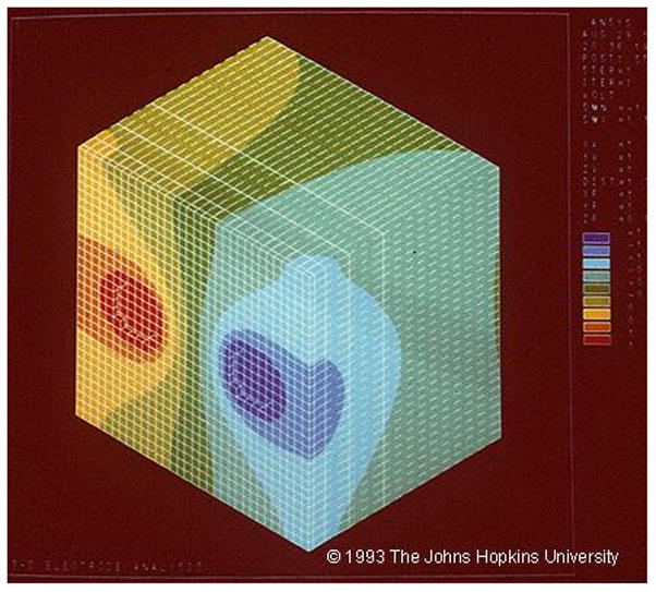
Finite element modeling, showing the normalized change in potential in response to current applied between a pair of adjacent electrodes, separated by 1 cm. The colors indicate normalized change in voltage, with red +1, blue -1. From Nathan et al., unpublished data, Fig. 4 is © 1993 The Johns Hopkins University. For more details on this, see Nathan et al. (1993a); Nathan et al. (1993b).
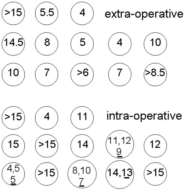
a) Comparison of extraoperative and intraoperative afterdischarge thresholds in a patient. During surgery, stimulation was as close as possible to the sites stimulated by the grid electrodes, doing this by placing ball electrodes directly over the subdural grid electrodes, then removing the grid, and placing the ball electrodes on the brain. In that patient extra-operative afterdischarge thresholds could vary by as much as 9.5 milliamperes and intraoperative thresholds by as much as 11 milliamperes between adjacent electrodes. The underlined numbers indicate thresholds 5 minutes after discontinuation of nitrous oxide. b) Intraoperative thresholds during functional testing in another patient. There was a 4.5 milliampere difference in functional thresholds between electrode pairs that were diagonally adjacent to one another. From Lesser et al., Epilepsia 25:615–621, 1984. With permission, Wiley-Blackwell (Lesser et al., 1984b).
a) Comparison of extraoperative and intraoperative afterdischarge thresholds in a patient. During surgery, stimulation was as close as possible to the sites stimulated by the grid electrodes, doing this by placing ball electrodes directly over the subdural grid electrodes, then removing the grid, and placing the ball electrodes on the brain. In that patient extra-operative afterdischarge thresholds could vary by as much as 9.5 milliamperes and intraoperative thresholds by as much as 11 milliamperes between adjacent electrodes. The underlined numbers indicate thresholds 5 minutes after discontinuation of nitrous oxide. b) Intraoperative thresholds during functional testing in another patient. There was a 4.5 milliampere difference in functional thresholds between electrode pairs that were diagonally adjacent to one another. From Lesser et al., Epilepsia 25:615–621, 1984. With permission, Wiley-Blackwell (Lesser et al., 1984b).
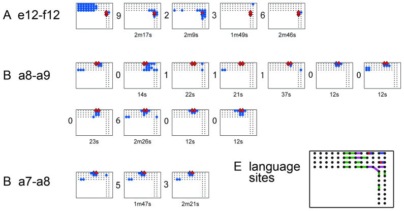
Afterdischarge responses at three stimulated electrode pairs. Within each of the three subfigures, each rectangle, with enclosed dots, blue circles and red diamonds, plots the location of afterdischarges after a single stimulation trial. Each subfigure shows all trials with afterdischarges due to stimulation of that electrode pair. There are numbers between each pair of plots. These numbers indicate how many trials without afterdischarges occurred between that pair of trials. The numbers under each plot indicate minutes (m) or seconds (s) between that trial and its predecessor. Red diamonds=stimulated pair. Blue circles=sites with afterdischarges. Responses vary in (A) and (B), whereas stimulation intensity remained stable. It was 15mA for all plots in (A), 14mA for all plots in (B). Responses vary little in (C), even though stimulation intensities did: 11, 14 and 13mA for plots 1, 2 and 3, respectively. Therefore, afterdischarge distribution is not explained by stimulation intensity alone. At times, plots can resemble one another, for example, the second and third plots in (A), and the last two plots in (B), but we saw no systematic overall pattern of recurrence, for example explainable by stimulation order or intensity. From: Lesser RP, Lee HW, Webber WR, Prince B, Crone NE, Miglioretti DL. Short-term variations in response distribution to cortical stimulation. Brain 2008 131:1528–1539, by permission of Oxford University Press.
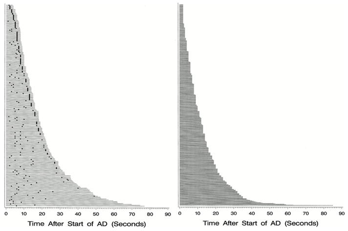
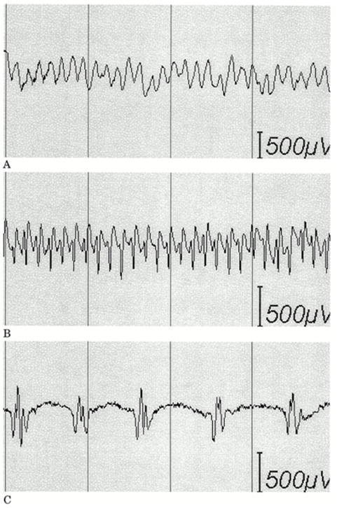
a) Afterdischarges (AD) occurred in this patient in response to stimulation. The two dots at the bottom indicate when each of two brief pulses of stimulation (BPS) were applied. The first was unsuccessful, but the second successful in stopping the afterdischarges. This method can terminate ADs, but works only about half the time, as shown in Fig. 7b. b) Duration and treatment latency of each individual trial during which a brief burst of pulse stimulation (BPS) was applied. Each horizontal line indicates a separate trial. The x-axis indicates the time after BPS application. The responses are arranged from top to bottom by total afterdischarge (AD) duration. Left: Duration of each individual trial during which BPS was applied. The dot represents the time that BPS was applied. The horizontal line extends 2 seconds past the dot in all cases because of blocking of the amplifier channels, lasting about two seconds after stimulation ended, during which time we could not know whether ADs were or were not continuing. Right: Duration of each individual trial during which BPS was not applied. BPS could stop ADs regardless of the treatment latency, might not stop ADs regardless of the treatment latency, and might stop spontaneously. However, ADs were significantly more likely to stop after BPS. c) Examples of types of afterdischarges that can occur in response to stimulation. (A) Continuous rhythmic epileptiform activity (epileptiform activity with an overall sinusoidal or semisinusoidal appearance); (B) rapidly repeated spikes without an overall appearance of a simple sinusoidal waveform; and (C) discrete individual spikes or polyspikes (discharges separated by at least several hundred milliseconds). Figures 7b and 7c are from Lesser RP, Kim SH, Beyderman L, Miglioretti DL, Webber WRS, Bare M, Cysyk B, Krauss G, and Gordon B. Brief bursts of pulse stimulation terminate afterdischarges caused by cortical stimulation. Neurology 1999. 53:2073–2081, with permission, Lippincott Williams & Wilkins.
a) Afterdischarges (AD) occurred in this patient in response to stimulation. The two dots at the bottom indicate when each of two brief pulses of stimulation (BPS) were applied. The first was unsuccessful, but the second successful in stopping the afterdischarges. This method can terminate ADs, but works only about half the time, as shown in Fig. 7b. b) Duration and treatment latency of each individual trial during which a brief burst of pulse stimulation (BPS) was applied. Each horizontal line indicates a separate trial. The x-axis indicates the time after BPS application. The responses are arranged from top to bottom by total afterdischarge (AD) duration. Left: Duration of each individual trial during which BPS was applied. The dot represents the time that BPS was applied. The horizontal line extends 2 seconds past the dot in all cases because of blocking of the amplifier channels, lasting about two seconds after stimulation ended, during which time we could not know whether ADs were or were not continuing. Right: Duration of each individual trial during which BPS was not applied. BPS could stop ADs regardless of the treatment latency, might not stop ADs regardless of the treatment latency, and might stop spontaneously. However, ADs were significantly more likely to stop after BPS. c) Examples of types of afterdischarges that can occur in response to stimulation. (A) Continuous rhythmic epileptiform activity (epileptiform activity with an overall sinusoidal or semisinusoidal appearance); (B) rapidly repeated spikes without an overall appearance of a simple sinusoidal waveform; and (C) discrete individual spikes or polyspikes (discharges separated by at least several hundred milliseconds). Figures 7b and 7c are from Lesser RP, Kim SH, Beyderman L, Miglioretti DL, Webber WRS, Bare M, Cysyk B, Krauss G, and Gordon B. Brief bursts of pulse stimulation terminate afterdischarges caused by cortical stimulation. Neurology 1999. 53:2073–2081, with permission, Lippincott Williams & Wilkins.
a) Afterdischarges (AD) occurred in this patient in response to stimulation. The two dots at the bottom indicate when each of two brief pulses of stimulation (BPS) were applied. The first was unsuccessful, but the second successful in stopping the afterdischarges. This method can terminate ADs, but works only about half the time, as shown in Fig. 7b. b) Duration and treatment latency of each individual trial during which a brief burst of pulse stimulation (BPS) was applied. Each horizontal line indicates a separate trial. The x-axis indicates the time after BPS application. The responses are arranged from top to bottom by total afterdischarge (AD) duration. Left: Duration of each individual trial during which BPS was applied. The dot represents the time that BPS was applied. The horizontal line extends 2 seconds past the dot in all cases because of blocking of the amplifier channels, lasting about two seconds after stimulation ended, during which time we could not know whether ADs were or were not continuing. Right: Duration of each individual trial during which BPS was not applied. BPS could stop ADs regardless of the treatment latency, might not stop ADs regardless of the treatment latency, and might stop spontaneously. However, ADs were significantly more likely to stop after BPS. c) Examples of types of afterdischarges that can occur in response to stimulation. (A) Continuous rhythmic epileptiform activity (epileptiform activity with an overall sinusoidal or semisinusoidal appearance); (B) rapidly repeated spikes without an overall appearance of a simple sinusoidal waveform; and (C) discrete individual spikes or polyspikes (discharges separated by at least several hundred milliseconds). Figures 7b and 7c are from Lesser RP, Kim SH, Beyderman L, Miglioretti DL, Webber WRS, Bare M, Cysyk B, Krauss G, and Gordon B. Brief bursts of pulse stimulation terminate afterdischarges caused by cortical stimulation. Neurology 1999. 53:2073–2081, with permission, Lippincott Williams & Wilkins.
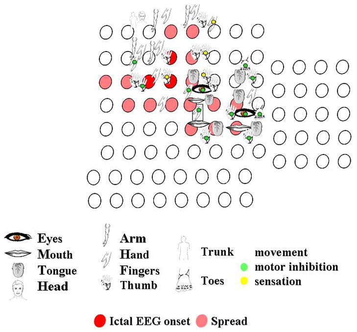
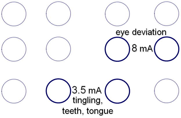
Responses to stimulation of the right peri-rolandic cortex. The figures indicate the body part stimulated. The green circle indicates that motor inhibition occurred, the yellow circle indicates where stimulation produced a sensory change. Other responses to stimulation were clonic or tonic movements. Each circle indicates an electrode. Circles filled red indicate where seizures began, those filled pink indicate seizure spread, in this patient with seizures originating in the motor cortex.
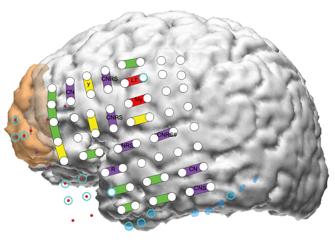
Results from mapping the left lateral neocortex. This is the same patient as shown in figure 3, and shows electrode placement during the second surgical admission. The brown area anteriorly indicates the first resection and the cross-hatched brown area the second cortical resection eventually performed. C, comprehension; L, lip; M, mouth; N, naming; R, reading; S, spontaneous speech; T, tongue; y, respiratory inhibition; #, psychic change but not typical seizure. Psychic changes were manifested by hearing voices during the first admission (electrode labelled CNRS#), by a feeling of separation. Upper case means a positive change, such as muscle twitching, or tingling sensation with stimulation. Lower case means negative change, such as inhibition of movement. With the exception of y, all motor and sensory findings were on the other side of the body. Reproduced from J Neurol Neurosurg Psychiat, Lee et al. 80:285–290, © 2009, with permission from BMJ Publishing Group Ltd.
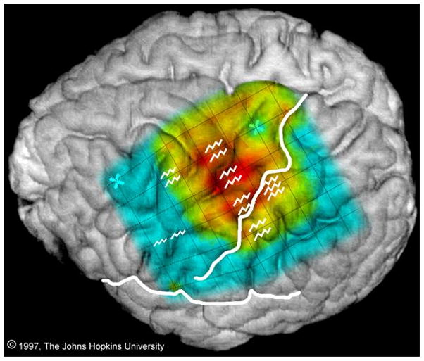
Comparison of sites where stimulation produced movement of the right arm or hand (jagged lines) with event-related spectral responses in the alpha band (power suppression, i.e. ERD, at 8–13 Hz) generated by finger wiggling. There is considerable overlap, but the sites are not identical. From: Crone NE, Miglioretti DL, Gordon B, Sieracki JM, Wilson MT, Uematsu S, and Lesser RP. Functional mapping of human sensorimotor cortex with electrocorticographic spectral analysis I. Alpha and beta event-related desynchronization. Brain 1998121:2271–2299, by permission of Oxford University Press.
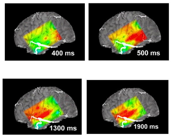
This figure diagrams the distribution of alpha suppression (ERD) during naming, as mapped using a subdural grid. The continuous color map is interpolated: actual data was from the 6x8 electrode array. The figure uses a standard “rainbow” color scale, where red indicates the greatest and blue the least suppression. At 400 and 500 msec suppression is present at the posterior inferior portion of the grid, perhaps during retrieval of the name of the object in the picture presented to the patient. At 1300 msec suppression is marked over the anterior-superior portion of the grid, perhaps corresponding to cortical control of articulation, and there is suppression over the more central portion of the grid, overlying the temporal auditory cortex, perhaps because the auditory system hears the word being articulated (self-speech). At 1900 msec alpha suppression is less marked anteriorly, but continues to be present in the central portion of the grid. See the Supplementary Videos S1 and S2 for animations of cortical responses during naming and auditory word repetition.
References
-
- Alarcon G, Binnie CD, Elwes RD, Polkey CE. Power spectrum and intracranial EEG patterns at seizure onset in partial epilepsy. Electroencephalogr Clin Neurophysiol. 1995;94:326–337. - PubMed
-
- Arroyo S, Lesser RP, Awad CA, Goldring S, Sutherling WW, Resnick TJ. Subdural and epidural grids and strips. In: Engel J Jr, editor. Surgical Treatment of the Epilepsies. Raven Press; New York: 1993. pp. 377–386.
-
- Arroyo S, Lesser RP, Gordon B, Jackson D. Mu rhythm in the human cortex: An electrophysiologic study with subdural electrodes. Neurology. 1992;42(Suppl 3):265. - PubMed
-
- Battaglia G, Chiapparini L, Franceschetti S, Freri E, Tassi L, Bassanini S, Villani F, Spreafico R, D'Incerti L, Granata T. Periventricular nodular heterotopia: classification, epileptic history, and genesis of epileptic discharges. Epilepsia. 2006;47:86–97. - PubMed
Publication types
MeSH terms
Grants and funding
LinkOut - more resources
Full Text Sources
Other Literature Sources
Medical
