A fast, angle-dependent, analytical model of CsI detector response for optimization of 3D x-ray breast imaging systems

Abstract

Purpose: Accurate models of detector blur are crucial for performing meaningful optimizations of three-dimensional (3D) x-ray breast imaging systems as well as for developing reconstruction algorithms that faithfully reproduce the imaged object anatomy. So far, x-ray detector blur has either been ignored or modeled as a shift-invariant symmetric function for these applications. The recent development of a Monte Carlo simulation package called MANTIS has allowed detailed modeling of these detector blur functions and demonstrated the magnitude of the anisotropy for both tomosynthesis and breast CT imaging systems. Despite the detailed results that MANTIS produces, the long simulation times required make inclusion of these results impractical in rigorous optimization and reconstruction algorithms. As a result, there is a need for detector blur models that can be rapidly generated.

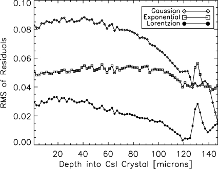
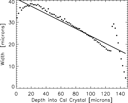
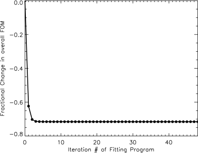
Methods: In this study, the authors have derived an analytical model for deterministic detector blur functions, referred to here as point response functions (PRFs), of columnar CsI phosphor screens. The analytical model is x-ray energy and incidence angle dependent and draws on results from MANTIS to indirectly include complicated interactions that are not explicitly included in the mathematical model. Once the mathematical expression is derived, values of the coefficients are determined by a two-dimensional (2D) fit to MANTIS-generated results based on a figure-of-merit (FOM) that measures the normalized differences between the MANTIS and analytical model results averaged over a region of interest. A smaller FOM indicates a better fit. This analysis was performed for a monochromatic x-ray energy of 25 keV, a CsI scintillator thickness of 150 microm, and four incidence angles (0 degrees, 15 degrees, 30 degrees, and 45 degrees).

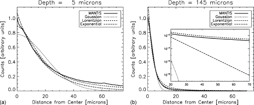
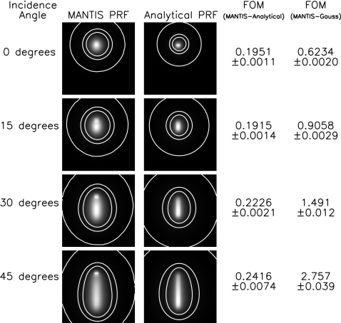
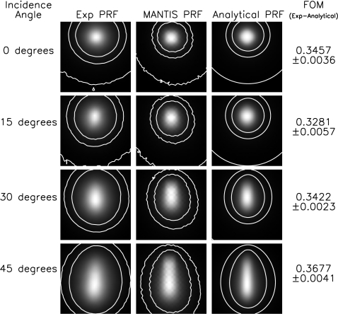
Results: The FOMs comparing the analytical model to MANTIS for these parameters were 0.1951 +/- 0.0011, 0.1915 +/- 0.0014, 0.2266 +/- 0.0021, and 0.2416 +/- 0.0074 for 0 degrees, 15 degrees, 30 degrees, and 45 degrees, respectively. As a comparison, the same FOMs comparing MANTIS to 2D symmetric Gaussian fits to the zero-angle PRF were 0.6234 +/- 0.0020, 0.9058 +/- 0.0029, 1.491 +/- 0.012, and 2.757 +/- 0.039 for the same set of incidence angles. Therefore, the analytical model matches MANTIS results much better than a 2D symmetric Gaussian function. A comparison was also made against experimental data for a 170 microm thick CsI screen and an x-ray energy of 25.6 keV. The corresponding FOMs were 0.3457 +/- 0.0036, 0.3281 +/- 0.0057, 0.3422 +/- 0.0023, and 0.3677 +/- 0.0041 for 0 degrees, 15 degrees, 30 degrees, and 45 degrees, respectively. In a previous study, FOMs comparing the same experimental data to MANTIS PRFs were found to be 0.2944 +/- 0.0027, 0.2387 +/- 0.0039, 0.2816 +/- 0.0025, and 0.2665 +/- 0.0032 for the same set of incidence angles.

Conclusions: The two sets of derived FOMs, comparing MANTIS-generated PRFs and experimental data to the analytical model, demonstrate that the analytical model is able to reproduce experimental data with a FOM of less than two times that comparing MANTIs and experimental data. This performance is achieved in less than one millionth the computation time required to generate a comparable PRF with MANTIS. Such small computation times will allow for the inclusion of detailed detector physics in rigorous optimization and reconstruction algorithms for 3D x-ray breast imaging systems.

Figure 1

Schematic of model geometry and coordinate system. The view is a vertical cut through the CsI crystal looking from the side with the air interface on the top and the detector layer at the bottom of the schematic. The infinitely thin incident x-ray beam enters at an angle of 90° minus θ from the x axis (ϕ, 90° minus the angle between the x-ray beam and the y axis, is assumed to be zero in this diagram). The y axis is going out of the page in this view.

Figure 2

Mass attenuation coefficient as a function of energy for CsI as simulated in PENELOPE. The photoelectric, Rayleigh, Compton, and total mass attenuation coefficients are shown. The photoelectric effect is the dominant interaction over the energy range of 5–100 keV.

Figure 3

Comparison of exponential x-ray absorption profile with a least-squares linear approximation for 25 keV. The exponential profile is indicated with a solid line and the linear approximation with a dashed line.

Figure 4

Percent of the emitted optical photons at a specific depth that reach the photodetector. Results from MANTIS simulations are shown as black dots, and a linear fit to that data is also shown. This information resulted in the use of a linear model for the crystal self-absorption.

Figure 5

Plots showing the normalized, radially averaged simulated optical-photon spread from MANTIS for two different depths; (left) 5 μm and (right) 145 μm with a zoom of the tails in the inset plot. The depth refers to the distance in the z direction between where the x-ray beam enters the CsI crystal and where the x ray is absorbed and produces the optical shower. The black lines show the radially averaged MANTIS results normalized to the maximum of the radially averaged profile. Fits of Gaussian, exponential, and Lorentzian functions are also shown. The Lorentzian shows the best overall fit to the data. In general, for optical photons produced deeper in the crystal, the Lorentzian tends to overestimate both the tails and the peak, while for shallower depths, it tends to underestimate both the tails and the peak.

Figure 6

Analysis to determine the functional form of the spread of optical photons that reach the detector after being generated at a specific depth. MANTIS simulated data were generated for depths in the crystal between 0 and 145 μm and Gaussian, exponential, and Lorentzian fits were performed to the radial average of the MANTIS results to determine the functional form of the spread. The RMS of the residuals of these fits are shown as a function of the depth at which the optical-photon shower was generated. The Lorentzian function gives the smallest RMS residuals for all depths.

Figure 7

FWHM of Lorentzian fits to MANTIS data as a function of depth where the optical photons were generated. The MANTIS data are shown as dots, while a linear fit is shown as a solid line. A linear relationship was used to model the width of the spread as a function of depth in the mathematical model.

Figure 8

Fractional change in the overall FOM during the 2D fitting process as a function of the iteration number of the fitting program. Data are shown for a 25 keV monochromatic incoming beam, 150 μm thick CsI screen, and the combination of 0°, 15°, 30°, and 45° incidence angles. The overall FOM stabilizes well before the end of the fitting procedure.

Figure 9

Comparison of MANTIS-generated PRFs with PRFs from the analytical model after the 2D fit. All PRFs have been generated with a CsI thickness of 150 μm and an x-ray energy of 25 keV. The incident x-ray beam is modeled in MANTIS as an infinitesimal pencil beam. The incidence angle of the x-ray beam is indicated in the leftmost column, followed by the corresponding MANTIS-generated PRFs, analytical model PRFs, FOMs from the comparison between the MANTIS and analytical PRFs, and, finally, the FOM from the comparison between MANTIS and 2D symmetric Gaussian fits to the normal incidence MANTIS PRF. All PRFs are 0.315×0.315 mm² with 9 μm pixels. Contours are shown for levels of 0.01, 0.05, and 0.1 times the maximum of the PRF.

Figure 10

Comparison of the analytical model with experimental PRFs. The experimental data were taken at 40 kVp (25.6 keV mean photon energy) with a 170 μm thick CsI scintillator and a 30 μm pinhole. The analytical model was convolved with a 30 μm incident beam profile and then fit to MANTIS data that were generated by taking into account all the details of the actual CsI screen geometry. The MANTIS data were generated with a 100 μm diameter pencil beam incident on a 30 μm pinhole. The incidence angle of the incoming x-ray beam is indicated in the leftmost column, followed by the corresponding experimental PRFs, MANTIS-generated PRFs, analytical model PRFs, and FOMs from the comparison between the experimental and the analytical data. The analytical model was fit to the MANTIS results then a comparison was performed between the analytical model and the experimental data. This procedure was followed as opposed to fitting the analytical model to the experimental data since experimental PRFs will not be available for typical applications. All PRFs are 0.315×0.315 mm² with 9 μm pixels. Contours are shown for levels of 0.01, 0.05, and 0.1 times the maximum of the PRF.

Figure 11

Line spread functions calculated from the PRFs presented in Fig. 10 (25.6 keV, 170 μm thick CsI). The PRFs were summed along the direction perpendicular to the incoming x-ray beam and then normalized by the maximum. Experimental data, MANTIS-generated PRFs, and analytical PRFs are plotted with solid, dashed, and dotted lines, respectively. Incidence angles of 0°, 15°, 30°, and 45° are presented from left to right. MANTIS tends to underestimate the width of the peak and overestimate the width of the tails. The analytical model matches MANTIS better than MANTIS matches the experimental data. The slight shift between the analytical model and the experimental data in the plot for 45° is due to the cross-correlation algorithm used to match the data. This provides the best match between the analytical and experimental PRFs when the entire PRF is taken into account.

References

1. Richard S. and Siewerdsen J. H., “Cascaded systems analysis of noise reduction algorithms in dual-energy imaging,” Med. Phys. MPHYA6 35(2), 586–601 (2008).10.1118/1.2826556 - DOI - PubMed
1. Yadava G. K., Kuhls-Gilcrist A. T., Rudin S., Patel V. K., Hoffmann K. R., and Bednarek D. R., “A practical exposure-equivalent metric for instrumentation noise in x-ray imaging systems,” Phys. Med. Biol. PHMBA7 53(18), 5107–5121 (2008).10.1088/0031-9155/53/18/017 - DOI - PMC - PubMed
1. Chen Y., Lo J. Y., and J. T.DobbinsIII, “Importance of point-by-point back projection correction for isocentric motion in digital breast tomosynthesis: Relevance to morphology of structures such as micro-calcifications,” Med. Phys. MPHYA6 34(10), 3885–3892 (2007).10.1118/1.2776256 - DOI - PubMed
1. Wu T., Moore R. H., Rafferty E. A., and Kopans D. B., “A comparison of reconstruction algorithms for breast tomosynthesis,” Med. Phys. MPHYA6 31(9), 2636–2647 (2004).10.1118/1.1786692 - DOI - PubMed
1. Badano A., Kyprianou I. S., Jennings R. J., and Sempau J., “Anisotropic imaging performance in breast tomosynthesis,” Med. Phys. MPHYA6 34(11), 4076–4091 (2007).10.1118/1.2779943 - DOI - PubMed
Publication types