Retinotopic mapping with spin echo BOLD at 7T

Abstract

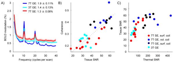
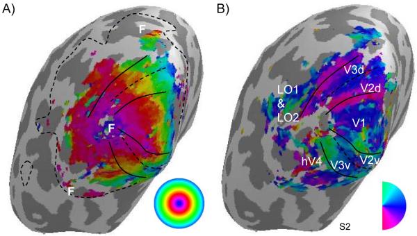
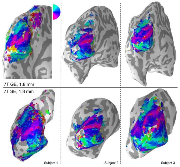
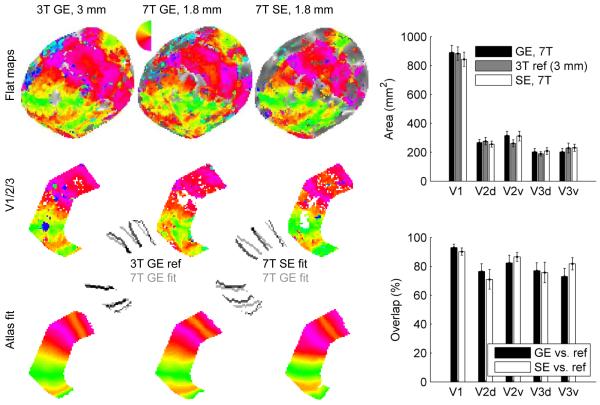
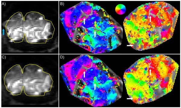
For blood oxygenation level-dependent (BOLD) functional MRI experiments, contrast-to-noise ratio (CNR) increases with increasing field strength for both gradient echo (GE) and spin echo (SE) BOLD techniques. However, susceptibility artifacts and nonuniform coil sensitivity profiles complicate large field-of-view fMRI experiments (e.g., experiments covering multiple visual areas instead of focusing on a single cortical region). Here, we use SE BOLD to acquire retinotopic mapping data in early visual areas, testing the feasibility of SE BOLD experiments spanning multiple cortical areas at 7T. We also use a recently developed method for normalizing signal intensity in T(1)-weighted anatomical images to enable automated segmentation of the cortical gray matter for scans acquired at 7T with either surface or volume coils. We find that the CNR of the 7T GE data (average single-voxel, single-scan stimulus coherence: 0.41) is almost twice that of the 3T GE BOLD data (average coherence: 0.25), with the CNR of the SE BOLD data (average coherence: 0.23) comparable to that of the 3T GE data. Repeated measurements in individual subjects find that maps acquired with 1.8-mm resolution at 3T and 7T with GE BOLD and at 7T with SE BOLD show no systematic differences in either the area or the boundary locations for V1, V2 and V3, demonstrating the feasibility of high-resolution SE BOLD experiments with good sensitivity throughout multiple visual areas.

Figure 1

Correction of intensity inhomogeneities in images allows for automated surface definition from high-field anatomical data. Top left: axial section from a T₁-weighted image (1 mm isotropic resolution) acquired with the 16-channel volume coil. Pattern of intensity non-uniformity is typical for 7T images acquired with transmit/receive coils, although systems with a separate transmit coil may produce less severe non-uniformities that may enable automated reconstruction without proton density normalization. Top middle: standard surface reconstruction software packages have a first-pass white-matter intensity correction stage (WM intensity correct), in which a coarse segmentation provides a low spatial frequency intensity filter. The non-uniformities are so strong, however, that these algorithms fail (white arrow). Top right: incomplete white matter definition makes it impossible to define a cortical surface (this segmentation was accomplished with SurfRelax; similar results were obtained with FreeSurfer). Bottom left: division by proton density scan (Ratio image) reduces intensity variations in white matter. The division generates some high-intensity noise at the perimeter of the brain, which can interfere with skull stripping but does not interfere with automated white matter surface definition. Bottom middle: corrected and normalized image, from which white matter can be segmented to define a full cortical surface (Bottom right). About an hour of manual editing was required to remove residual errors in white matter definition for superior temporal and inferior frontal regions; the same problems are commonly seen in 3T acquisitions.

Figure 2

Correction of intensity inhomogeneities in images enables automated surface definition and inflation for partial brain anatomical data acquired at 7T. A) A “proton density” scan shows the sensitivity profile of the surface coil, positioned here to cover early visual areas. B) The raw T₁ anatomy has the expected non-uniformity in intensity, but the corrected image shown here (MP-RAGE divided by proton density) has uniform contrast throughout posterior cortex, up to the limit where coil SNR is insufficient. C) The cortical surface is reconstructed by finding the boundary between white matter and gray matter. The intensity-based algorithm relies on uniform white matter intensity throughout the cortical region. D) The final product is an inflated white matter surface. Light gray shading indicates regions of positive curvature (gyri); dark gray indicates negative curvature (sulci).

Figure 3

Fourier spectra and contrast-to-noise ratios estimated from the retinotopic mapping experiment. A) Average amplitude spectra for all 1.8 mm acquisitions. All subjects participated in the 7T mapping sessions (7T GE data for subjects 1-3 was acquired with a volume coil, 7T GE data for subjects 4-6 was acquired with a surface coil; all 7T SE data was acquired with a surface coil); Subjects 3-6 participated in the high-resolution 3T mapping session. Data for each experiment are averaged regions of interest defined as subsets of V1 from approximately 2 to 6 degrees eccentricity (an average of 345 voxels per hemisphere). BOLD contrast was characterized by the amplitude of modulation at 10 cycles per scan. B) Average tissue SNR (mean intensity divided by standard deviation through time for each voxel) was calculated for each hemisphere of each subject. Stimulus coherence is the unsigned correlation between the BOLD data and a sinusoid at 10 cycles per scan. A strong linear correlation was observed between coherence and tissue SNR (dotted line). C) Thermal SNR was calculated as the mean voxel intensity divided by average standard deviation (through time) in a noise ROI defined outside the brain.

Figure 4

Spin echo retinotopic data from one subject illustrates the coverage achieved in this experiment, as well as the basic organization of early visual areas. The phase of the stimulus-related Fourier component (encoding visual field location, as indicated by inset legends) is visualized on inflated cortical surfaces reconstructed from anatomical images acquired with a surface coil. A) The eccentricity map is the average of four scans. No smoothing was used for the functional data; data are shown for voxels with coherence greater than 0.3 (p < 0.001, uncorrected). Dashed line indicates extent of coverage for functional data; coverage was sufficient for early visual areas, but was not sufficient to fully visualize maps sharing foveal representations (marked with F) on the dorsal and ventral surfaces of the brain. B) Early visual areas are marked on the polar angle map derived from the rotating wedge functional scans.

Figure 5

Retinotopic maps for three hemispheres. Top row: retinotopic maps acquired with gradient echo BOLD at 7T (1.8 mm resolution, average of 2 4-minute scans), visualized on whole-brain cortical surfaces reconstructed from anatomical images acquired with a volume coil at 7 Tesla. Bottom row: retinotopic maps acquired with spin echo BOLD (1.8 mm resolution, average of 6 4-minute scans), visualized on partial-brain cortical surfaces acquired with a surface coil. (To the extent allowed by the different shapes of the different inflated hemispheres, the partial hemispheres are viewed from the same angle as the complete hemispheres, but the perspective could not be perfectly matched.) For all datasets, functional data from voxels with coherence > 0.30 are visualized on inflated surfaces, except for the SE data from Subject 1, for which voxels with co > 0.25 are shown. Missing data due to errors in alignment between functional and anatomical data are apparent as holes in the color overlay.

Figure 6

Atlas-fitting quantifies visual area boundaries. At left, atlas fitting is illustrated for Subject 3, right hemisphere. Top row: data are visualized on flat patches from the same (3T) reference anatomy. Because not all of the subjects who participated in the 7T studies participated in the 3T high-resolution mapping study, 3T GE BOLD retinotopic mapping data with 3 mm resolution is used as the reference. Middle row: sub-region of V1/2/3 extending from approximately 2-6 degrees eccentricity, for which atlas-fitting was performed. Bottom row: phase atlases created for each hemisphere after warping to match the phase data. Phase reversals in these warped atlases define visual area boundaries, which are indicated by the inset gray lines. A comparison between 3T and 7T GE map boundaries is shown in the left inset; a comparison of 7T GE and SE map boundaries is shown in the right inset. The bar chart at upper right indicates the average area (n=12 hemispheres, errorbars indicate SEM) of the restricted eccentricity band for each visual area, for each modality. The bar chart on the lower right indicates, for the 7T GE and SE data sets, what percentage of voxels in each visual area were also contained in the corresponding visual area defined by the 3T reference data.

Figure 7

Correction of image distortion due to field inhomogeneities improves visualization of retinotopic maps from functional data acquired at 7T. A) The raw distorted EPI image; yellow reference line shows true brain boundary as measured by anatomical data. Blue arrow indicates a region of particularly strong distortion. B) Left and right hemisphere maps from a single subject, before distortion compensation. Functional data are shown on flattened cortical patches; legend in the middle indicates color code for visual field position. C) Residual distortion is still apparent in distortion-compensated images, as the “corrected” EPI data still do not perfectly match the anatomical reference. D) Functional data from the distortion-compensated images is nevertheless more consistently represented on the reconstructed cortical surface, both because of improved alignment between functional and anatomical data and better fidelity of shape. White arrows indicate regions of particular improvement.

References

1. Ugurbil K, Adriany G, Andersen P, et al. Ultrahigh field magnetic resonance imaging and spectroscopy. Magn Reson Imaging. 2003;21(10):1263–1281. - PubMed
1. Yacoub E, Shmuel A, Pfeuffer J, et al. Imaging brain function in humans at 7 Tesla. Magn Reson Med. 2001;45(4):588–594. - PubMed
1. Yacoub E, Duong TQ, Van de Moortele P-F, et al. Spin-echo fMRI in humans using high spatial resolutions and high magnetic fields. Magnetic Resonance in Medicine. 2003;49:655–664. - PubMed
1. Vaughan JT, Garwood M, Collins CM, et al. 7T vs. 4T: RF power; homogeneity; and signal-to-noise comparison in head images. Mag Reson Med. 2001;46:24–30. - PubMed
1. Thulborn KR, Waterton JC, Matthews PM, Radda GK. Oxygenation dependence of hte transverse relaxation time of water protons i nwhole blood at high field. Biochimica et Biophysica Acta - General Subjects. 1982;714(2):265–270. - PubMed
Publication types