. 2010 Jul 15;6(7):e1000856.
doi: 10.1371/journal.pcbi.1000856.

Do humans optimally exploit redundancy to control step variability in walking?

Affiliations

Do humans optimally exploit redundancy to control step variability in walking?

Jonathan B Dingwell et al. PLoS Comput Biol. .

Abstract

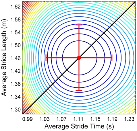
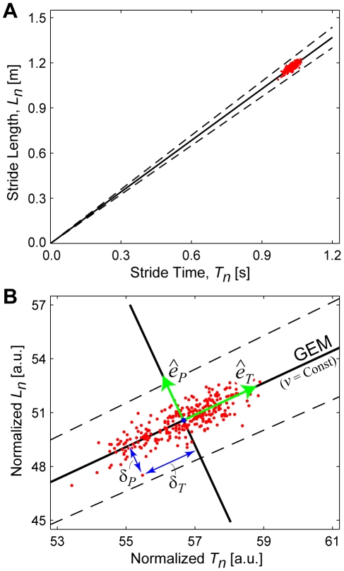
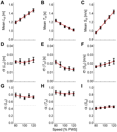
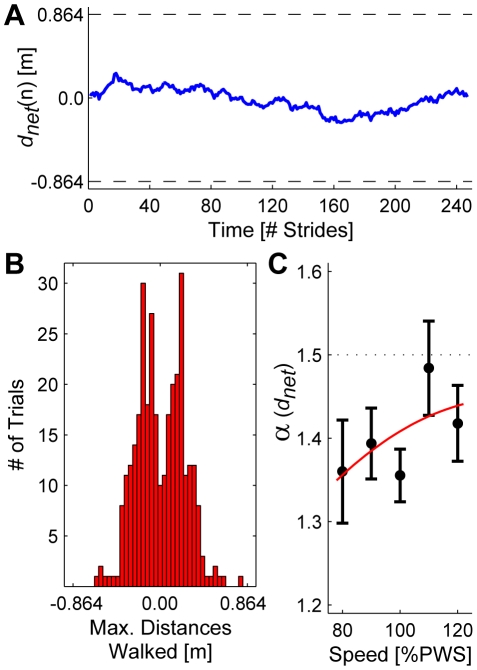
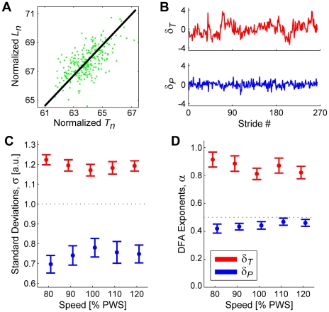
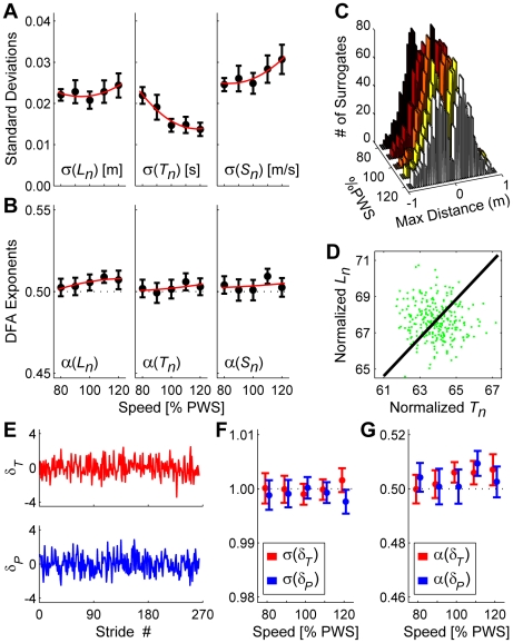
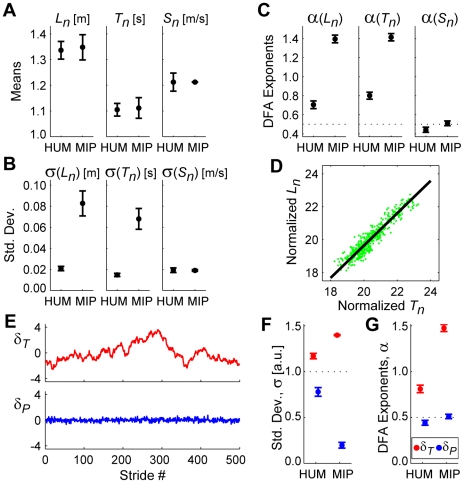
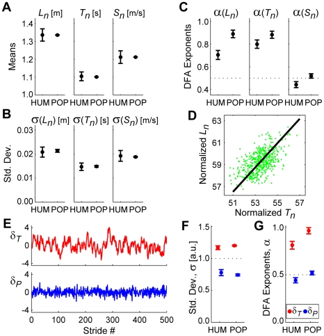
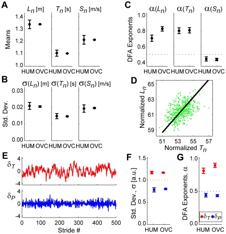
It is widely accepted that humans and animals minimize energetic cost while walking. While such principles predict average behavior, they do not explain the variability observed in walking. For robust performance, walking movements must adapt at each step, not just on average. Here, we propose an analytical framework that reconciles issues of optimality, redundancy, and stochasticity. For human treadmill walking, we defined a goal function to formulate a precise mathematical definition of one possible control strategy: maintain constant speed at each stride. We recorded stride times and stride lengths from healthy subjects walking at five speeds. The specified goal function yielded a decomposition of stride-to-stride variations into new gait variables explicitly related to achieving the hypothesized strategy. Subjects exhibited greatly decreased variability for goal-relevant gait fluctuations directly related to achieving this strategy, but far greater variability for goal-irrelevant fluctuations. More importantly, humans immediately corrected goal-relevant deviations at each successive stride, while allowing goal-irrelevant deviations to persist across multiple strides. To demonstrate that this was not the only strategy people could have used to successfully accomplish the task, we created three surrogate data sets. Each tested a specific alternative hypothesis that subjects used a different strategy that made no reference to the hypothesized goal function. Humans did not adopt any of these viable alternative strategies. Finally, we developed a sequence of stochastic control models of stride-to-stride variability for walking, based on the Minimum Intervention Principle. We demonstrate that healthy humans are not precisely "optimal," but instead consistently slightly over-correct small deviations in walking speed at each stride. Our results reveal a new governing principle for regulating stride-to-stride fluctuations in human walking that acts independently of, but in parallel with, minimizing energetic cost. Thus, humans exploit task redundancies to achieve robust control while minimizing effort and allowing potentially beneficial motor variability.


Conflict of interest statement

The authors have declared that no competing interests exist.

Figures

Figure 1
Figure 1. Predicted metabolic cost as a function of average stride length (L) and average stride time (T).
Contour lines represent iso-energy level curves for average energetic cost of transport: i.e., energy expenditure per distance walked per kg of body mass (cal/m/kg). The optimum (i.e., minimal) cost [TOpt, LOpt] occurs at the center of the figure. These contours were determined from the empirical equations derived by Zarrugh et al. . Representative results are shown for the nominal gait pattern of one typical subject, after subtracting the metabolic cost of standing . The diagonal black line represents the line of constant speed, v, which passes through [TOpt, LOpt]. Horizontal and vertical error bars indicate the energetic consequences of ±7% errors in either T or L, respectively. These are similar in amplitude to ±3 standard deviations in each of these variables, as observed experimentally (Fig. 3D–E), and thus approximate the general range of stride-to-stride variations expected to be observed in these measures. The horizontal and vertical axes are likewise scaled to ±12% change in each variable. These iso-energy contours are nearly isotropic: i.e., relative changes in stride length incur nearly the same energetic cost penalty as comparable relative changes in stride time. (See Supplementary Text S1 for additional details).
Figure 2
Figure 2. Schematic representation of the goal equivalent manifold (GEM) for walking.
(A) Example stride time and stride length data. Each dot represents the particular combination of stride length (Ln) and stride time (Tn) for one individual stride. The solid diagonal line defines the set of all combinations of Ln and Tn that achieve the exact same speed, v. This line is the Goal Equivalent Manifold (GEM) for walking (Eq. 2) at constant speed v. The dashed diagonal lines represent ±5% error in maintaining this constant speed. (B) To facilitate the analyses, we non-dimensionalize the data by normalizing the Ln and Tn time series each to unit variance. We then re-define the goal function and the GEM accordingly. We define orthonormal basis vectors, [êT, êP], aligned tangent to and perpendicular to the GEM, respectively. We then transform the dimensionless Ln and Tn time series into δT and δP time series of deviations in the êT and êP directions, respectively, relative to the mean operating point, [T*, L*], along the GEM. Note that the GEM is defined by the average walking speed as set by the treadmill and is therefore independent of how data points representing individual strides are distributed within the [Tn, Ln] plane. The GEM exists prior to and independent of any notions of how people actually control their stride-to-stride movements with respect to it (if at all).
Figure 3
Figure 3. Primary gait parameters.
Means (A, B, C), standard deviations (σ: D, E, F), and DFA exponents (α: G, H, I), for stride length (Ln), stride time (Tn), and stride speed (Sn) as a function of walking speed from 80% to 120% of preferred walking speed (PWS). Error bars indicate between-subject ±95% confidence intervals at each speed. At faster walking speeds, subjects adopted longer stride lengths (A) and faster stride times (B). The variability in stride length (D) remained similar across speeds, while the variability in stride times (E) decreased at faster walking speeds. Consequently, the variability in the stride speeds (F) increased slightly at faster walking speeds. Subjects exhibited significant stride-to-stride statistical persistence (i.e., α>>½) in both stride lengths (G) and stride times (H), suggesting that deviations in these measures were not immediately corrected on consecutive strides. Conversely, subjects consistently exhibited slight anti-persistence (i.e., α<½) in stride speeds (I), suggesting that this measure of walking performance was under tighter control. Note: Linear trend lines in (A)–(C) and quadratic trend lines in (D)–(I) are shown only to provide a visual reference.
Figure 4
Figure 4. Absolute distances walked on the treadmill.
(A) Net cumulative distance, dnet(n), walked (i.e., absolute position, Eq. 6) on the treadmill over time for a typical trial for a typical human subject. Dashed horizontal lines at ±0.864 m indicate the front and back limits of the treadmill belt. All subjects exhibited substantial deviations in absolute position that were sustained across multiple strides, consistent with previous findings , , , . (B) Histogram of maximum rearward (−) and forward (+) distances walked by each subject during each trial at all 5 speeds (166 total trials). Histograms for each individual speed looked similar. Note that most subjects did not get close to reaching the treadmill belt limits (±0.864 m). (C) These stride-to-stride shifts in absolute treadmill position exhibited very strong statistical persistence,approaching that of Brownian motion (i.e., integrated white noise: α = 1.5), particularly at the faster walking speeds. Thus, these deviations in absolute position were not tightly controlled. Note: the vertical scale here is quite different from Fig. 3G–I. The quadratic trend line is shown only to provide a visual reference.
Figure 5
Figure 5. GEM decomposition results.
(A) Example GEM data from a typical subject. Individual dots represent individual strides. The diagonal line represents the GEM (see Fig. 2). (B) Time series of δT and δP deviations for the data set shown in (A). Qualitatively, the δT deviations exhibit larger amplitudes and also appear to show greater statistical persistence than the δP deviations. (C) Standard deviations for all δT and δP time series at all 5 walking speeds. Error bars represent between-subject ±95% confidence intervals. Subjects exhibited significantly greater variability along the GEM (δT) than perpendicular to the GEM (δP): F(1,16) = 139.93; p = 2.53×10⁻⁹. (D) DFA α exponents for all δT and δP time series at all 5 walking speeds. Error bars represent between-subject ±95% confidence intervals. Subjects exhibited significantly greater statistical persistence along the GEM (δT) than perpendicular to the GEM (δP): F(1,16) = 368.21; p = 1.81×10⁻¹². Additionally, all subjects exhibited significant anti-persistence (95% confidence interval upper bounds all <½) for the goal-relevant δP deviations at all 5 walking speeds.
Figure 6
Figure 6. Independently randomly shuffled surrogate walking.
All error bars represent between-subject ±95% confidence intervals. By definition, these surrogates exhibited the same mean stride parameters (not shown) as the original walking data (Fig. 3AC ). (A) These surrogates exhibited the same Ln and Tn variability as the original data (Fig. 3DE ). However, Sn variability increased slightly (compare to Fig. 3F ). (B) Unlike the experimental trials (Fig. 3GI ), these surrogates exhibited no strong temporal correlations (all α≈½) for any of the basic stride parameters (Note, the vertical scale is very different from Fig. 3GI ). (C) Histograms of maximum forward and backward distances walked by all 20 surrogates for each trial. By construction, no surrogate walked beyond either the front or back edges of the treadmill belt (i.e., ±0.864 m). (D) A typical surrogate for the trial shown in Fig. 5A . The GEM (diagonal line) remains the same. However, the distribution of strides around the GEM is now approximately isotropic. (E) Time series of δT and δP deviations for the surrogate trial shown in (D). Neither time series exhibited obvious persistence. (F) Variability (σ) for δT and δP deviations from the GEM was not significantly different (F(1,16) = 2.614; p = 0.125) (Compare to Fig. 5C and note the different vertical scales). (G) There were no strong temporal correlations (α≈½) for either δT or δP deviations and α's for both directions were not different from each other (F(1,16) = 0.413; p = 0.529) (Compare to Fig. 5D and note the different vertical scales).
Figure 7
Figure 7. Stochastically optimal minimum intervention principle (MIP) model for step regulation.
All error bars represent between-subject ±95% confidence intervals. In (A)–(C) and (F)–(G), HUM data are the experimental data from Fig. 3 for 100% PWS. (A) Mean stride lengths (Ln), times (Tn) and speeds (Sn) for humans (HUM) and for the MIP model (MIP). (B) Within-subject standard deviations for Ln, Tn, and Sn. (C) DFA exponents (α) for Ln, Tn, and Sn. (D) A typical trial for the MIP model. The diagonal line represents the GEM. As expected, the distribution of strides is very tightly compressed along the GEM. (E) Time series of δT and δP deviations for the trial shown in (D). Note the substantial statistical persistence exhibited by the δT time series. (F) Variability (σ) for the MIP model data was significantly greater for δT deviations than for δP deviations (F(1,39) = 6,076.51; p = 1.53×10−43). The MIP model exhibited much greater δT variability and much less δP variability than did human subjects (HUM). (G) DFA exponents (α) for the MIP model were significantly larger for δT deviations than for δP deviations (F(1,39) = 1,969.18; p = 2.40×10⁻³⁴). DFA exponents (α) for δT deviations were ∼1.5, reflecting Brownian motion (i.e., statistical diffusion) along the GEM. Conversely, α exponents for the δP deviations were ∼½, reflecting nearly uncorrelated fluctuations. These goal-relevant δP deviations did not exhibit the anti-persistent behavior seen in the experimental data (Fig. 5D ).
Figure 8
Figure 8. Stochastically optimal MIP-based model with “preferred operating point” (POP) for step regulation.
All error bars represent between-subject ±95% confidence intervals. In (A)–(C) and (F)–(G), HUM data are the experimental data from Fig. 3 for 100% PWS. (A) Mean stride lengths (Ln), times (Tn) and speeds (Sn) for humans (HUM) and for the POP model. (B) Within-subject standard deviations for Ln, Tn, and Sn. (C) DFA exponents (α) for Ln, Tn, and Sn. (D) A typical POP model trial. The diagonal line represents the GEM. As expected, the distribution of strides is not nearly as compressed along the GEM as for the MIP model (Fig. 7D ). (E) Time series of δT and δP deviations for the trial shown in (D). The δT time series appears to exhibit persistence. The δP time series does not. (F) Variability (σ) for the POP model was still greater for δT deviations than for δP deviations (F(1,39) = 2,916.30; p = 1.55×10−37). However, the variance ratio, σ(δT)/σ(δP), was much closer that of humans. (G) DFA exponents (α) for the POP model were significantly larger for δT deviations than for δP deviations (F(1,39) = 597.27; p = 7.61×10⁻²⁵). For δT deviations, these α were still >1.0, reflecting substantial statistical persistence. Likewise, the α for δP deviations were still ∼½, reflecting uncorrelated fluctuations. The δP deviations still did not exhibit the anti-persistent behavior seen experimentally (Fig. 5D ).
Figure 9
Figure 9. Sub-optimal MIP-based model with “over-correcting” (OVC) controller for step regulation.
All error bars represent between-subject ±95% confidence intervals. In (A)–(C) and (F)–(G), HUM data are the experimental data from Fig. 5 for 100% PWS. (A) Mean stride lengths (Ln), times (Tn) and speeds (Sn) for humans (HUM) and OVC model (OVC). (B) Within-subject standard deviations for Ln, Tn, and Sn. (C) DFA exponents (α) for Ln, Tn, and Sn. (D) A typical OVC model trial. The diagonal line represents the GEM. The distribution of strides with respect to the GEM appears similar to the POP model (Fig. 8D ) and to humans (Fig. 5A ). (E) Time series of δT and δP deviations for the trial shown in (D). The δP time series now appears to exhibit slightly more rapid fluctuations than did the POP model (Fig. 8E ). (F) Variability (σ) for the OVC model was much greater for δT deviations than for δP deviations (F(1,39) = 1,736.81; p = 2.49×10⁻³³). The variance ratio, σ(δT)/σ(δP), was again very similar to humans. (G) DFA exponents (α) for the OVC model were significantly larger for δT deviations than for δP deviations (F(1,39) = 713.02; p = 3.15×10⁻²⁶). Deviations along the GEM (δT) again exhibited statistical persistence. Conversely, the δP deviations consistently exhibited α<½. Thus, these δP deviations did exhibit the anti-persistent behavior seen experimentally (Fig. 5D ).

References

    1. Zehr EP, Stein RB. What Functions do Reflexes Serve During Human Locomotion? Prog Neurobiol. 1999;58:185–205. - PubMed
    1. Warren WH, Kay BA, Zosh WD, Duchon AP, Sahuc S. Optic Flow is Used to Control Human Walking. Nat Neurosci. 2001;4:213–216. - PubMed
    1. Bent LR, Inglis JT, McFadyen BJ. When is Vestibular Information Important During Walking? J Neurophysiol. 2004;92:1269–1275. - PubMed
    1. Rossignol S, Dubuc R, Gossard J-P. Dynamic Sensorimotor Interactions in Locomotion. Physiol Rev. 2006;86:89–154. - PubMed
    1. Margaria R. Sulla fisiologia, e specialmente sul consumo energetico, della marcia e della corsa a varie velocita ed inclinazioni del terreno. Accad Naz Lincei Rc. 1938;6 7:299–368.

Publication types