. 2011 Sep;32(9):1383-99.
doi: 10.1002/hbm.21114. Epub 2010 Aug 5.

Modeling of the human skull in EEG source analysis

Affiliations

Modeling of the human skull in EEG source analysis

Moritz Dannhauer et al. Hum Brain Mapp. 2011 Sep.

Abstract

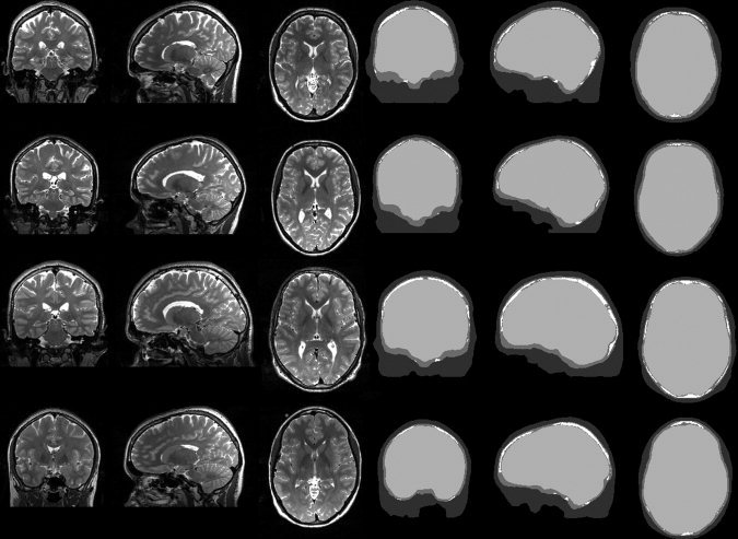
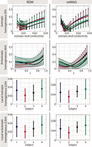
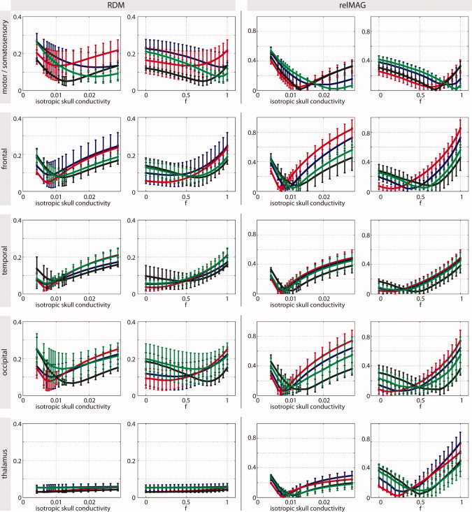
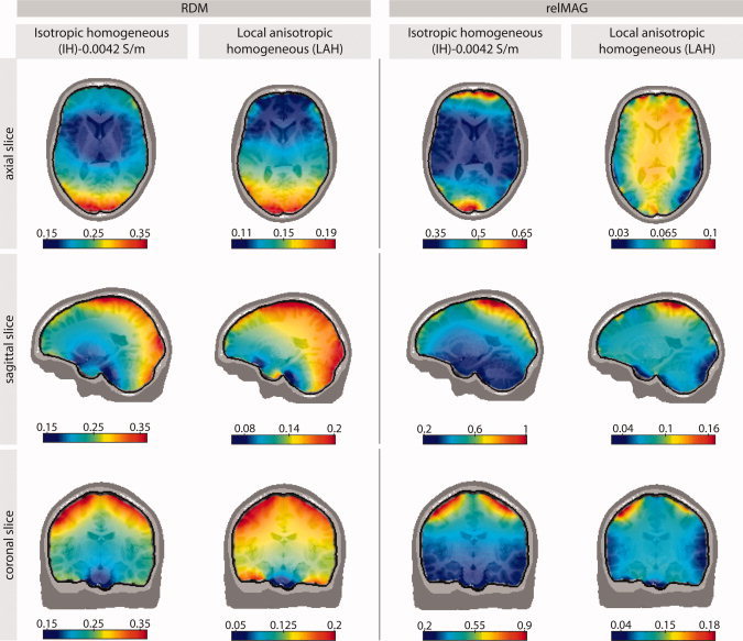
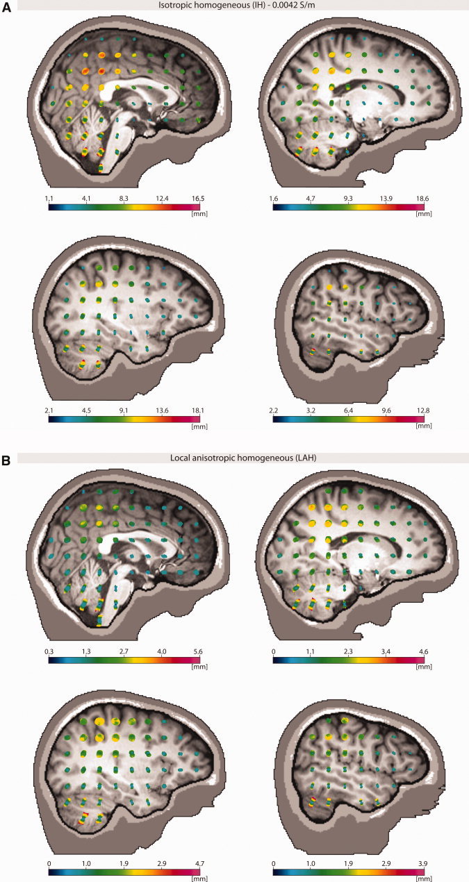
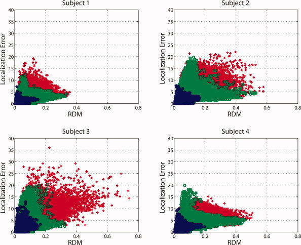
We used computer simulations to investigate finite element models of the layered structure of the human skull in EEG source analysis. Local models, where each skull location was modeled differently, and global models, where the skull was assumed to be homogeneous, were compared to a reference model, in which spongy and compact bone were explicitly accounted for. In both cases, isotropic and anisotropic conductivity assumptions were taken into account. We considered sources in the entire brain and determined errors both in the forward calculation and the reconstructed dipole position. Our results show that accounting for the local variations over the skull surface is important, whereas assuming isotropic or anisotropic skull conductivity has little influence. Moreover, we showed that, if using an isotropic and homogeneous skull model, the ratio between skin/brain and skull conductivities should be considerably lower than the commonly used 80:1. For skull modeling, we recommend (1) Local models: if compact and spongy bone can be identified with sufficient accuracy (e.g., from MRI) and their conductivities can be assumed to be known (e.g., from measurements), one should model these explicitly by assigning each voxel to one of the two conductivities, (2) Global models: if the conditions of (1) are not met, one should model the skull as either homogeneous and isotropic, but with considerably higher skull conductivity than the usual 0.0042 S/m, or as homogeneous and anisotropic, but with higher radial skull conductivity than the usual 0.0042 S/m and a considerably lower radial:tangential conductivity anisotropy than the usual 1:10.


Figures

Figure 1
Figure 1
Representative MR slices (left panel) and segmentation results (right panel) for the four subjects (numbering ascending from top to bottom). Color coding of segmentation: dark gray—skin, mid gray—compact skull tissue, white—spongy skull tissue, light gray—interior of skull (CSF, brain gray and white matter, etc.).
Figure 2
Figure 2
Generalized errors in forward computation. The errors were computed between the respective simplified skull model (IH, AH, LIH, and LAH) and the reference model (IMC). For the IH and AH models, we varied the conductivity and the relative spongy bone proportion, respectively. The colors represent the four different subjects. Results were averaged over all dipoles in the brain. Error bars denote standard deviations. [Color figure can be viewed in the online issue, which is available at wileyonlinelibrary.com.]
Figure 3
Figure 3
Errors in forward computation for specific brain areas (global models only). The errors were computed between the respective simplified skull model (IH and AH) and the reference model (IMC). We varied the conductivity and the relative spongy bone proportion, respectively. The colors represent the four different subjects. Error bars denote standard deviations. [Color figure can be viewed in the online issue, which is available at wileyonlinelibrary.com.]
Figure 4
Figure 4
Spatial distribution of average (over all four subjects) forward modeling errors plotted on selected MRI slices of one subject (subject 1). Column 1 depicts the RDM errors of the IH model with the conventionally used skull conductivity value of 0.0042 S/m with respect to the IMC (reference) model. Column 2 shows the RDM error of the LAH model, which in general appeared to be the best approximation of the IMC model (see Fig. 2). Columns 3–4 show the relMAG error, respectively. [Color figure can be viewed in the online issue, which is available at wileyonlinelibrary.com.]
Figure 5
Figure 5
(A) The localization errors are plotted as a function of both dipole position and dipole orientation using glyph plots. For visualization, the glyph is color‐coded with the localization error. We analyzed these models which, for the forward solutions, turned out to be worst (largest difference with reference model), that is the IH (isotropic homogeneous, with conductivity 0.0042 S/m). (B) The localization errors are plotted as a function of both dipole position and dipole orientation using glyph plots. For visualization, the glyph is color‐coded with the localization error. We analyzed these models which, for the forward solutions, turned out to be best (closest agreement with reference model), that is the LAH (local anisotropic) model. [Color figure can be viewed in the online issue, which is available at wileyonlinelibrary.com.]
Figure 6
Figure 6
Forward topography error (RDM) and inverse (localization) error interaction depicted individually for each subject. The local models are depicted as blue dots. The optimized models and the standard model (IH, 0.0042 S/m) are shown as green circles and red crosses, respectively. [Color figure can be viewed in the online issue, which is available at wileyonlinelibrary.com.]

Similar articles

Cited by

References

    1. Akhtari M, Bryant HC, Marnelak AN, Flynn ER, Heller L, Shih JJ, Mandelkern M, Matlachov A, Ranken DM, Best ED, DiMauro MA, Lee RR, Sutherling WW ( 2002): Conductivities of three‐layer live human skull. Brain Topography 14: 151–167. - PubMed
    1. Awada KA, Jackson DR, Williams JT, Wilton DR, Baumann SB, Papanicolaou AC ( 1997): Computational aspects of finite element modeling in EEG source localization. IEEE Trans Biomed Eng 44: 736–752. - PubMed
    1. Baysal U, Haueisen J ( 2004): Use of a priori information in estimating tissue resistivities—Application to human data in vivo. Physiol Meas 25: 737–748. - PubMed
    1. Bertrand O (1991): 3D Finite element method in brain electrical activity studies. In Nenonen J, Rajala HM, Katila T. (Eds.) (1991): Biomegnetic localization and 3D Modeling, pp. 154–171, Helsinki University of Technology, Helsinki, Finnland.
    1. Braess D (2007): Finite Elements: Theory, Fast Solvers, and Applications in Solid Mechanics, Cambridge University Press; 3 edition (April 30, 2007), ISBN‐10: 0521705185, ISBN‐13: 978‐0521705189.

Publication types