Encoding and decoding in fMRI

Abstract

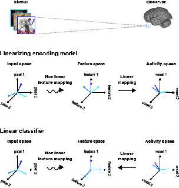
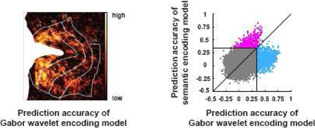
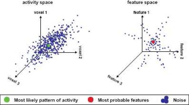
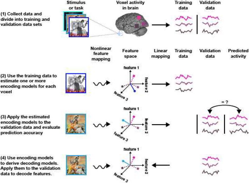
Over the past decade fMRI researchers have developed increasingly sensitive techniques for analyzing the information represented in BOLD activity. The most popular of these techniques is linear classification, a simple technique for decoding information about experimental stimuli or tasks from patterns of activity across an array of voxels. A more recent development is the voxel-based encoding model, which describes the information about the stimulus or task that is represented in the activity of single voxels. Encoding and decoding are complementary operations: encoding uses stimuli to predict activity while decoding uses activity to predict information about the stimuli. However, in practice these two operations are often confused, and their respective strengths and weaknesses have not been made clear. Here we use the concept of a linearizing feature space to clarify the relationship between encoding and decoding. We show that encoding and decoding operations can both be used to investigate some of the most common questions about how information is represented in the brain. However, focusing on encoding models offers two important advantages over decoding. First, an encoding model can in principle provide a complete functional description of a region of interest, while a decoding model can provide only a partial description. Second, while it is straightforward to derive an optimal decoding model from an encoding model it is much more difficult to derive an encoding model from a decoding model. We propose a systematic modeling approach that begins by estimating an encoding model for every voxel in a scan and ends by using the estimated encoding models to perform decoding.

Figure 1. Linearizing encoding and decoding models

[Top] The brain can be viewed as a system that nonlinearly maps stimuli into brain activity. According to this perspective a central task of systems and cognitive neuroscience is to discover the nonlinear mapping between input and activity. [Middle] Linearizing encoding model. The relationship between encoding and decoding can be described in terms of a series of abstract spaces. In experiments using visual stimuli the axes of the input space are the luminance of pixels and each point in the space (here different colors in the input space) represents a different image. Brain activity measured in each voxel is represented by an activity space. The axes of the activity space correspond to the activity of different voxels and each point in the space represents a unique pattern of activity across voxels (different colors in the activity space). In between the input and activity spaces is a feature space. The mapping between the input space and the feature space is nonlinear and the mapping between the feature space and activity space is linear. [Bottom] Linear classifier. The linear classifier is a simple decoding model that can also be described in terms of input, feature and activity spaces. However, the direction of the mapping between activity and feature space is reversed relative to the encoding model. Because the features are discrete all points in the feature space lie along the axes

Figure 2. Comparative analyses using encoding models

[Left] Prediction accuracy for a Gabor wavelet encoding model. The stimuli used in the experiment were grayscale natural scenes. A Gabor wavelet encoding model was estimated for each voxel. Here the prediction accuracy for each voxel has been projected onto a digitally flattened map of visual cortex. Known visual areas are outlined in white. Prediction accuracy for the Gabor wavelet model is highest in early visual areas such as primary visual cortex, and declines in higher areas. Maps such as this one can be used to compare the representation of a specific set of features (such as Gabor wavelets) across many regions of interest. [Right] Comparison of prediction accuracy for two different encoding models. The horizontal axis gives prediction accuracy for the Gabor wavelet encoding model shown at left. The vertical axis gives prediction accuracy for a semantic encoding model. Each dot indicates an individual voxel. Cyan dots indicate voxels that are better modeled by the Gabor wavelet encoding model while magenta dots indicate voxels that are better modeled by the semantic encoding model. Gray dots indicate voxels that are not modeled well by either of these two encoding models. The two models provide good predictions for different populations of voxels. As this figure shows, it is easy to compare the accuracy of predictions for distinct encoding models even when the models are based upon very different features. In contrast, it is difficult to compare predictions of decoding models that decode different features.

Figure 3. Encoding and decoding distributions

[Left] The encoding distribution describes variance in the patterns of activity (blue dots) that are evoked by repeated presentations of the same stimulus. It also describes the location of the most likely pattern of activity (green dot) given the stimulus. A perfect encoding model would be able to predict the most likely pattern of activity evoked by any arbitrary stimulus. [Right] The decoding distribution describes variance in the features (blue dots) that evoke the same pattern of activity. It also describes the most probable features (red dot) given the pattern of activity. Maximum a posteriori decoding attempts to predict the most probable feature, given any arbitrary pattern of activity.

Figure 4. The combined encoding / decoding approach

The relationship between encoding and decoding models suggests an ideal procedure for analyzing fMRI data that consists of four steps (one step for each row in the figure). [Row 1] Voxel activity (jagged lines) evoked by experimental stimuli (scenes at left) is divided into a training data set and a validation data set. [Row 2] Encoding models are specified by a nonlinear mapping (curvy arrow) of the stimuli into an abstract feature space (labeled axes represent hypothetical feature space; stimuli depicted by line with circular end). Model weights (dashed lines with square ends) estimated from training data specify a linear mapping (straight arrows) from feature space to voxel activity. [Row 3] Prediction accuracy is measured by comparing the activity in the validation data set to the predicted activity (far right). [Row 4] Decoding models are derived by using Bayes’ theorem to reverse the direction of the linear mapping (straight arrow).

References

1. Adelson EH, Bergen JR. Spatiotemporal energy models for the perception of motion. J. Opt. Soc. Am. A. 1985;2(2):284–299. - PubMed
1. Aertsen A, Johannesma P. The spectro-temporal receptive field. A functional characteristic of auditory neurons. Biol. Cybern. 1981;42(2):133–143. - PubMed
1. Beauchamp MS, LaConte S, Yasar N. Distributed representation of single touches in somatosensory and visual cortex. Hum. Brain Mapp. 2009;30(10):3163–3171. - PMC - PubMed
1. Bishop CM. Pattern recognition and machine learning. Springer; New York: 2006.
1. Bredfeldt CE, Ringach DL. Dynamics of spatial frequency tuning in macaque V1. J. Neurosci. 2002;22:1976–1984. - PMC - PubMed