Psychophysical reverse correlation with multiple response alternatives

Abstract

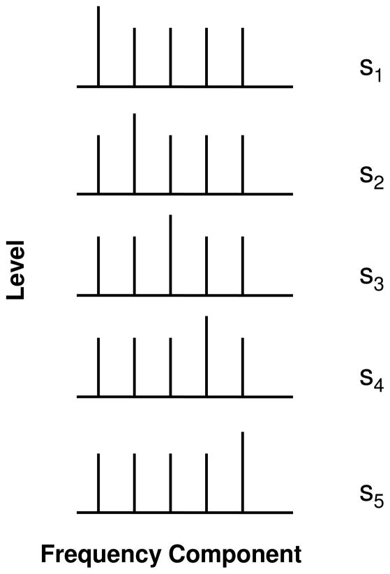
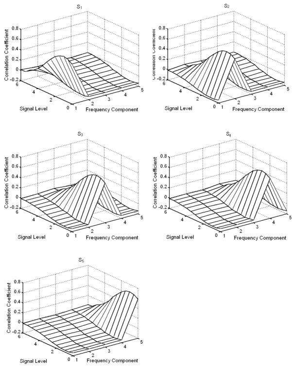
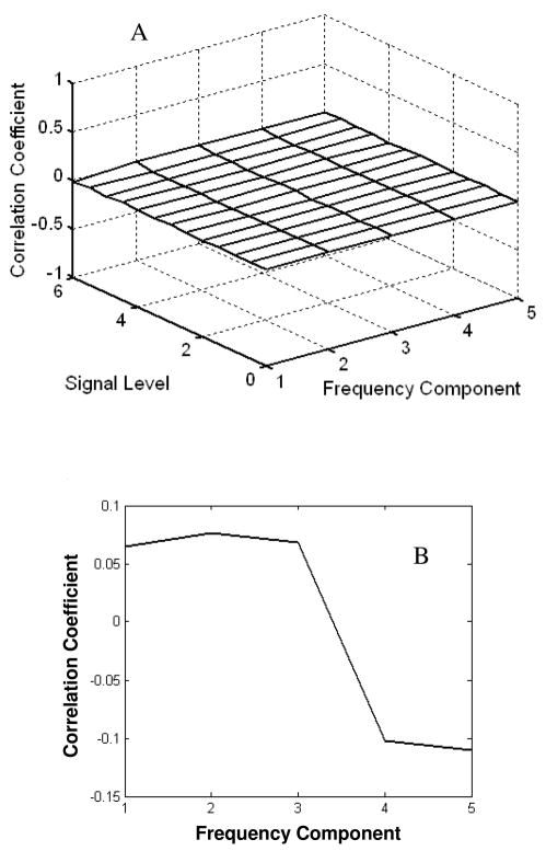
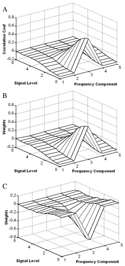
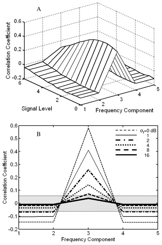
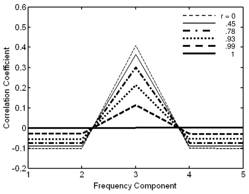
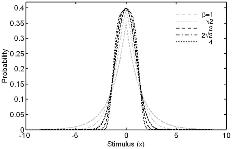
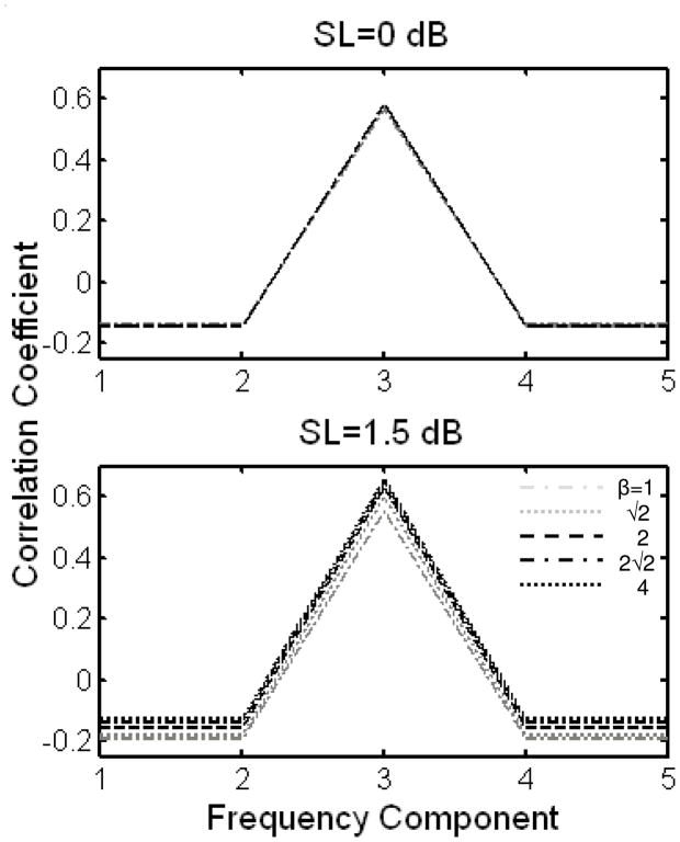
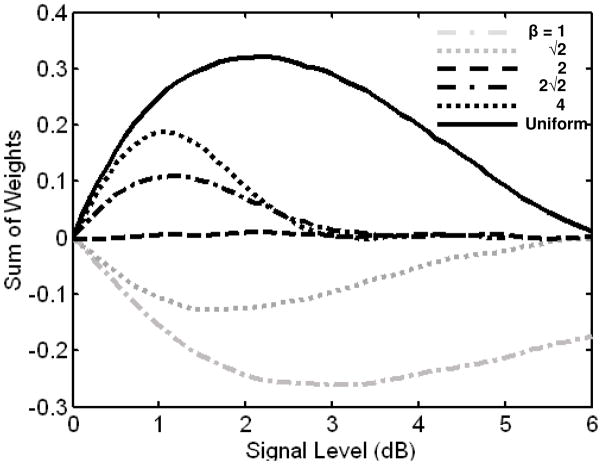
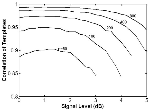
Psychophysical reverse-correlation methods such as the "classification image" technique provide a unique tool to uncover the internal representations and decision strategies of individual participants in perceptual tasks. Over the past 30 years, these techniques have gained increasing popularity among both visual and auditory psychophysicists. However, thus far, principled applications of the psychophysical reverse-correlation approach have been almost exclusively limited to two-alternative decision (detection or discrimination) tasks. Whether and how reverse-correlation methods can be applied to uncover perceptual templates and decision strategies in situations involving more than just two response alternatives remain largely unclear. Here, the authors consider the problem of estimating perceptual templates and decision strategies in stimulus identification tasks with multiple response alternatives. They describe a modified correlational approach, which can be used to solve this problem. The approach is evaluated under a variety of simulated conditions, including different ratios of internal-to-external noise, different degrees of correlations between the sensory observations, and various statistical distributions of stimulus perturbations. The results indicate that the proposed approach is reasonably robust, suggesting that it could be used in future empirical studies.

Figure 1

Spectra of the five stimuli used in the spectral-shape identification experiment. Each spectrum consists of five components. The level of one component is increased by DL (dB) relative to that of the other components. The five resulting stimuli are denoted S₁ to S₅, with the digit indicating the rank of the incremented component.

Figure 2

Estimated weighting patterns, or identification templates, of a simulated optimal observer in an m-alternative identification task involving the stimuli shown in Figure 1. The weight estimates are given by point-biserial correlation coefficients between the series of perturbations applied to the levels of the stimulus components, and the corresponding series of response scores (1 for correct, 0 for incorrect), across all trials on which a given stimulus (indicated above each panel) was presented. The coefficients are plotted as a function of the stimulus component number (from 1 to 5), and of the signal strength; the latter was controlled by the increment (DL) applied to the level of the target stimulus component, and varied from 0 to 6 dB.

Figure 3

Influence of indiscriminate across-trial averaging on estimated weighting patterns. A. “Overall” weighting pattern estimated by pooling all trials together in the simulated spectral-shape identification experiment involving the five stimuli illustrated in Figure 1. B. Weighting pattern obtained by pooling data across all trials in a simulated spectral-shape identification experiment involving only the first three of the five stimuli shown in Figure 1, i.e., S₁, S₂, and S₃. In these simulations, the signal strength (controlled by the level increment, DL, applied to the target stimulus component) was set to 0 dB.

Figure 4

Example response-based weighting patterns and “classification images”. A. Response-based weighting patterns based on point-biserial correlation coefficients calculated across all trials between the random perturbations applied to the stimulus-component levels and a binary variable, which was equal to 1 when the response was “S₃”, and to 0 otherwise. B. Classification image obtained by averaging stimulus–levels perturbations across all trials on which the response was “S₃”, regardless of which stimulus alternative was actually presented. To facilitate comparison with the panel S₃ in Figure 2, the weights were scaled by a constant factor so that, for a signal strength (DL) of 0 dB, the weight of the middle component was equal in the two figures. C. Classification image obtained by averaging the random perturbations applied to stimulus-component levels across all trials on which the response was different from “S₃”, regardless of which stimulus alternative was actually presented. These weights were scaled by the same factor as in panel B.

Figure 5

Influence of internal noise on measured weighting patterns. A. Example 3-D weighting pattern obtained in simulations involving internal noise with a standard deviation equal to that of the external perturbations (1 dB). This 3-D weighting pattern is for stimulus S₃; it can be compared with that shown in the panel labeled “S₃” in Figure 2, which was obtained with no internal noise. B. Changes in weighting patterns with increasing amounts of internal noise. The different lines indicate weighting patterns obtained in simulations involving internal noise with a standard deviation of 0, 1, 2, 4, 8, or 16 dB, as indicated by the legend. The shaded area around zero correlation represents the 95% confidence interval around a correlation coefficient of zero based on 2000 trials. Only the weighting patterns measured using a null signal strength (DL = 0 dB) is shown here. Note that in this and subsequent figures, only the weighting pattern for stimulus S₃ (i.e., the stimulus with the middle component increased) is shown; the weighting patterns for other stimuli can be obtained from the one shown here by rearranging the frequency-component ranks so that the largest weights correspond to the target component.

Figure 6

Influence of correlations between the sensory observations on measured weighting functions. The different line types indicate different degrees of correlation between the target and non-target components: 0, 0.45, 0.78, 0.93, 0.99, and 1. The shaded area around zero correlation represents the 95% confidence interval around a correlation coefficient of zero based on 2000 trials.

Figure 7

Probability distributions of stimulus perturbations used in the simulations. These functions were produced by varying the exponent, β, in the function: $p(x)=\kappa e^{-{\mid \frac{x}{\sqrt{2}}\mid }^{\beta }}$. This exponent determines the kurtosis of the distribution. The curves are for β=1 (Laplace, grey-dashed line), √2, 2 (Gaussian, dark-dashed line), 2√2, and 4 (dark-dotted line), from leptokurtic to platykurtic.

Figure 8

Measured weighting functions in simulations using the distributions of perturbations shown in Figure 7. A. Results for a signal strength, DL, of 0 dB. B. Results for a signal strength, DL, of 1.5 dB. The line-style code is the same as in the previous figure.

Figure 9

Influence of the distribution of perturbations on the sum of measured weights as a function of signal strength (controlled by the size of the increment applied to the level of the target stimulus component). Except for the solid line, which corresponds to a uniform distribution, the line-style code is the same as in the previous figure.

Figure 10

Mean Pearson correlation coefficients between optimal templates, and templates estimated based on Monte Carlo simulations involving different numbers of trials, ranging from 50 to 800. The correlation coefficients are shown as a function of signal strength (DL), with the number of simulated trials as the parameter; the latter is indicated next to each curve. Each point in this figure represents a mean across 1,000 stochastic simulations.

References

-
- Abbey CK, Eckstein MP. Classification image analysis: estimation and statistical inference for two-alternative forced-choice experiments. Journal of Vision. 2002;2:66–78. - PubMed
- Ahumada AJ., Jr Classification image weights and internal noise level estimation. Journal of Vision. 2002;2:121–131. - PubMed
- Ahumada AJJ. Perceptual classification images from vernier acuity masked by noise. Perception. 1996;26:18.
- Ahumada AJJ, Beard BL. Response classification images in vernier acuity. Investigations in Opthalmology and Visual Science. 1998;40:S572.
- Ahumada AJJ, Lovell J. Stimulus features in signal detection. Journal of the Acoustical Society of America. 1971;49:1751–1756.
Publication types
MeSH terms
Grants and funding
LinkOut - more resources
Full Text Sources
Miscellaneous