Higher-order correlations in non-stationary parallel spike trains: statistical modeling and inference

Abstract

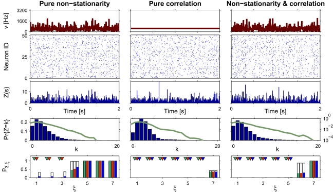
The extent to which groups of neurons exhibit higher-order correlations in their spiking activity is a controversial issue in current brain research. A major difficulty is that currently available tools for the analysis of massively parallel spike trains (N >10) for higher-order correlations typically require vast sample sizes. While multiple single-cell recordings become increasingly available, experimental approaches to investigate the role of higher-order correlations suffer from the limitations of available analysis techniques. We have recently presented a novel method for cumulant-based inference of higher-order correlations (CuBIC) that detects correlations of higher order even from relatively short data stretches of length T = 10-100 s. CuBIC employs the compound Poisson process (CPP) as a statistical model for the population spike counts, and assumes spike trains to be stationary in the analyzed data stretch. In the present study, we describe a non-stationary version of the CPP by decoupling the correlation structure from the spiking intensity of the population. This allows us to adapt CuBIC to time-varying firing rates. Numerical simulations reveal that the adaptation corrects for false positive inference of correlations in data with pure rate co-variation, while allowing for temporal variations of the firing rates has a surprisingly small effect on CuBICs sensitivity for correlations.

Keywords: higher-order correlations; multiple unit activity; non-stationarity; statistical population model.

Figure 1

Schema of the compound Poisson process and its measurement. Left: spike event times (horizontal bars) of individual neurons x₁(t),…,x_N(t) and tick marks of the carrier process z(t) (top) with the associated amplitudes (numbers above the ticks). The population spike count Z(s) (below the spike trains) counts the number of spikes across all neurons in bins of width h (dotted lines). Right: distributions of the amplitudes a_j, f_A (top) and of the population spike counts, f_Z, (bottom; blue bars: f_Z from 100 s of data with the given amplitude distribution, estimated using a bin size of h = 5 ms; dashed line: Poisson fit, corresponding to an independent population with the same firing rates). To construct a population of correlated spike trains, amplitudes a_j are drawn for all events t_j in the carrier process i.i.d from f_A. Individual processes x_i(t) are constructed by assigning subsequent events of the carrier process z(t) into a_j “child” processes x_i(t) (here, events are assigned randomly to the specific process IDs). Correlations of order ξ are induced, whenever events in the carrier process are copied into more than ξ processes, i.e., if the amplitude distribution assigns non-zero probabilities for amplitudes ≥ ξ.

Figure 2

Non-stationarities in the CPP. Panels (A–C) show carrier rates ν(t) in Hz (top panels), the distributions of the bin-wise mean carrier rates (“carrier distributions” f_R, small panels on the right; bin size h = 20 ms), the event-times of the carrier process z(t) (second panels from top), raster plots (third panels from top) and population spike counts Z(s) (bottom panels) for three different data sets. (A) Time varying assignment distribution produces non-stationary single processes, although the carrier process z(t) is stationary (constant carrier rate ν(t) = 50 Hz; all carrier events with t_j < 1 s are assigned randomly, all carrier events with t_j ≥ 1 and amplitude a_j = 1 are assigned to neuron 3). (B) Cosine carrier rate results in non-stationary carrier process z(t), the subsequent uniform assignment to N = 25 neurons generates a homogeneous, non-stationary population. (C) The carrier rate is constant in bins of length h = 20 ms and subsequent values of ν(t) are i.i.d. realizations with the carrier distribution of the cosine carrier rate in (B). Carrier events in (C) are assigned uniformly to N = 50 neurons. As illustrated by the virtually identical population spike count distributions shown in (D) (estimated from 1000 s of artificial data, color code as in B,C; note logarithmic y-scale), the differences in both the carrier rate, in particular the temporal order of the bins, and the assignment, in particular the number of neurons of the generated population, do not influence the statistics of the population spike count Z. (E) Amplitude distributions of all three data sets are superpositions of a “background-peak” at ξ = 1 and a binomial distribution B(10,0.3) (color code as in A–C).

Figure 3

Population statistics and CuBIC results for cosine-like non-stationarity for three data sets. Shown are the carrier rate ν(t) (top panels), raster plots of N = 50 spike trains (second panels from top) and population spike counts Z(s) obtained with a bin width of length h = 5 ms (third panels from top) for the first 2 s of a data stretch of length T = 100 s. Below are the empirical distributions f_Z(k) = Pr{Z = k} estimated from the entire data set (second panel from bottom; blue bars: linear y-scale with axes on the left, green solid line: logarithmic y-scale with axes on the right). Bottom panels show p-values of the stationary CuBIC (green), the adapted CuBIC with cosine-like rate variations (red) and with bimodal rate variations (blue), where rejected null-hypotheses, i.e., p-values below a significance level of α = 0.05, are marked by arrowheads. Outlined bars and arrowheads in bottom panel show results of data where interspike intervals below 2 ms were removed before the analysis. Data with pure rate non-stationarity (left column) have a sinusoidal carrier rate ν(t) (top panel) and an amplitude distribution with mass concentrated at ξ = 1 (f_A(k) = 0 for k > 1; see text for details). Pure correlation (middle column) is modeled with a stationary carrier rate and correlation up to order 7 (ν(t) = const., f_A(k) = 0 for k∉{1,7}). The probability for the high-amplitude events results in a pairwise correlation coefficient of c = 0.01 if the events of the carrier process are distributed uniformly among the processes N = 50. The combined data set with non-stationarity and correlation (right column) has the same correlation structure as the data in the middle column, and the same carrier rate as in the first column.

Figure 4

Population statistics and CuBIC results for non-stationarities with gamma-distributed carrier rate. The figure has the same setup as Figure 3, only that the bottom panels show results for stationary CuBIC (green bars and arrowheads), allowed uniform carrier distribution (red bars and arrowheads) and gamma-distributed carrier rate (blue bars and arrowheads).

Figure 5

Results of the maximization (Eq. 25 with appropriate objective functions) for data with pure correlation (see legend of Figure 3 for parameters). (A) Normalized variance of the rate variable ${\beta }_2^{\ast }$ that solves Eq. 25 for ξ = 1,…,7 for different types of allowed non-stationarities (green: stationary CuBIC; red: non-stationary CuBIC allowing uniform carrier distribution; blue: non-stationary CuBIC allowing gamma carrier distribution). (B) The maximal third cumulant ${\kappa }_{3,\xi }^{\ast }$ as a function of the test parameter ξ for different types of allowed non-stationarities (same color code as in A). Error bars denote $2\sqrt{\text{Var}\left[k_3\right]},$ corresponding to a significance level of α ≈ 0.05, the dashed line is the value of the test statistic k₃ and arrowheads denote rejected null-hypothesis where ${\text{κ}}_{3,\text{ξ}}^{\text{*}}+2\sqrt{\text{Var}\left[k_3\right]}<k_3$ (compare bottom panel of middle column in Figure 4).

References

-
- Abeles M. (1991). Corticonics: Neural Circuits of the Cerebral Cortex, 1st Edn.Cambridge: Cambridge University Press
- Aertsen A., Gerstein G., Habib M., Palm G. (1989). Dynamics of neuronal firing correlation: modulation of “effective connectivity”. J. Neurophysiol. 61, 900–917 - PubMed
LinkOut - more resources
Full Text Sources