Lifetime-based tomographic multiplexing

Abstract

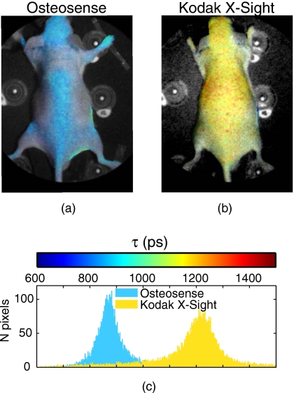
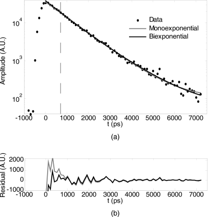
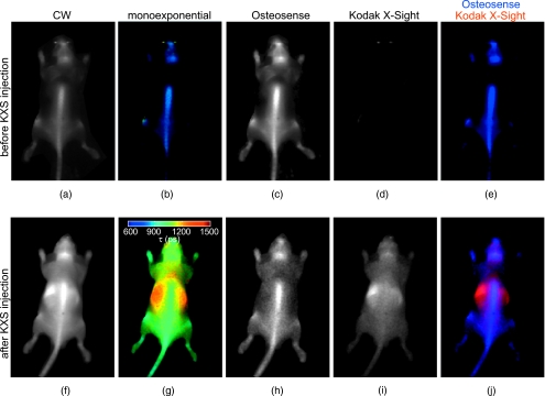
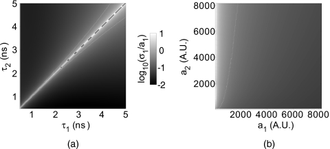
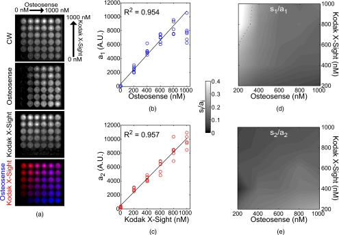
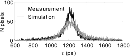
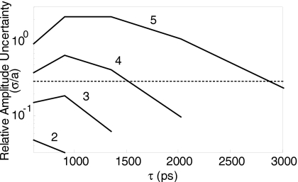
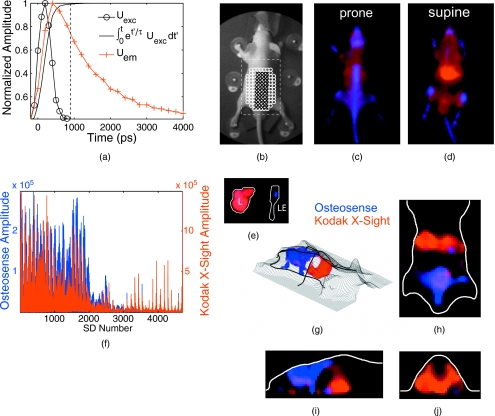
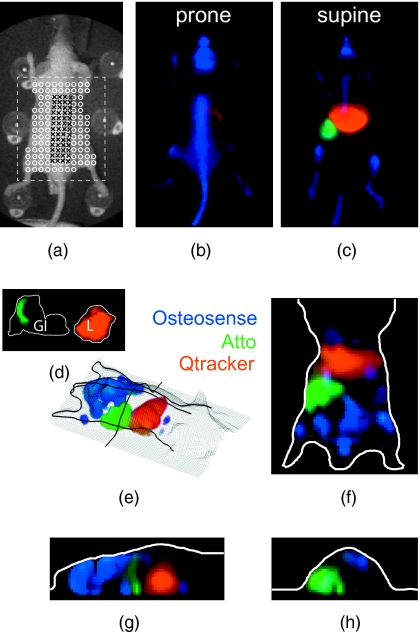
Near-infrared (NIR) fluorescence tomography of multiple fluorophores has previously been limited by the bandwidth of the NIR spectral regime and the broad emission spectra of most NIR fluorophores. We describe in vivo tomography of three spectrally overlapping fluorophores using fluorescence lifetime-based separation. Time-domain images are acquired using a voltage-gated, intensified charge-coupled device (CCD) in free-space transmission geometry with 750 nm Ti:sapphire laser excitation. Lifetime components are fit from the asymptotic portion of fluorescence decay curve and reconstructed separately with a lifetime-adjusted forward model. We use this system to test the in vivo lifetime multiplexing suitability of commercially available fluorophores, and demonstrate lifetime multiplexing in solution mixtures and in nude mice. All of the fluorophores tested exhibit nearly monoexponential decays, with narrow in vivo lifetime distributions suitable for lifetime multiplexing. Quantitative separation of two fluorophores with lifetimes of 1.1 and 1.37 ns is demonstrated for relative concentrations of 1:5. Finally, we demonstrate tomographic imaging of two and three fluorophores in nude mice with fluorophores that localize to distinct organ systems. This technique should be widely applicable to imaging multiple NIR fluorophores in 3-D.

Figure 1

In vivo lifetime characteristics of commercially available NIR fluorophores. Mice were administered NIR fluorophores and imaged for up to 1 day to determine biodistribution and in vivo fluorescence lifetimes. Planar fluorescence images were thresholded and each pixel was fit for a monoexponential decay. Monoexponential lifetime maps for (a) Osteosense and (b) Kodak X-Sight 761, overlaid on a white light planar reflectance image of the mouse. (c) Histogram of pixel lifetime values from (a) and (b). The two fluorophores have distinct, separable lifetimes in vivo.

Figure 2

Mono- versus biexponential analysis. (a) A single pixel data point from an in vivo measurement of two fluorophores (Osteosense 750 and Kodak X-Sight 761) was fit for either a single lifetime (monoexponential, resultant τ=1054) or for two a-priori lifetimes (biexponential, τ₁=835 ps and τ₂=1343). All data points after the dashed line (representing the time gate for fitting t_d) were included in the fit. (b) Residuals from fits in (a).

Figure 3

Planar fluorescence lifetime imaging of Osteosense 750 and Kodak X-Sight 761. A nude mouse received 2-nmol Osteosense 24 h prior to imaging; planar fluorescence time-resolved images were collected immediately before [(a) through (e)] and after [(f) to (j)] administration of Kodak X-Sight 761 (3 nmol). Image pixels were fit for the amplitude and lifetime of a monoexponential function, or were fit for a biexponential function with known lifetime components (see Fig. 2). (a) and (f) Continuous wave (cw) images. (b) and (g) Lifetime maps from monoexponential fit; color bar indicates the lifetime colormap. (c) and (h) Osteosense 750 lifetime component (τ₁=835 ps) from biexponential fit. (d) and (i) Kodak X-Sight 761 lifetime component (τ₂=1343 ps). (e) and (j) RGB images with Osteosense component in blue and Kodak X-Sight in red.

Figure 4

Noise considerations for lifetime unmixing. Lifetime recovery was simulated assuming Poisson statistics, i.e., ${\sigma }_y^2=\beta y+{\sigma }_r^2$, with β=6.53 and a dynamic range of 2¹⁴ (4×4 hardware and 2×2 software binning). (a) Relative amplitude uncertainty for equal amplitude probes of lifetimes τ₁ and τ₂. (b) Relative amplitude uncertainty of the first amplitude component for varying amplitudes a₁ and a₂ over the dynamic range of the instrument, with fixed lifetimes τ₁=1 ns and τ₂=1.2 ns. The white lines in (a) and (b) indicate the 30% relative uncertainty contours.

Figure 5

Multiwell separation of Osteosense and Kodak X-Sight. A multiwell plate was filled with Osteosense and Kodak X-Sight in orthogonal axes, from 0 to 1000 nM, in 200-nM steps. The multiwell plate was imaged in planar fluorescence mode, and subsequent images were fit for the lifetime components of 1126 (a₁, Osteosense) and 1376 ps (a₂, Kodak X-Sight), which were obtained from wells containing only a single fluorophore. (a) cw and recovered amplitude components of the multiwell plate. In the biexponential frame (bottom), Kodak X-Sight is in red, Osteosense is in blue. (b) and (c) Recovered component amplitudes (arbitrary units, AU) and linear fit to fluorophore concentration; correlation is shown in top left of each graph. (d) and (e) Amplitude uncertainty (s_i∕a_i), for (d) Osteosense and (e) Kodak X-Sight. (Color online only.)

Figure 6

Noise propagation to τ. The effects of measurement noise on the estimation of τ were determined by simulating a measurement of Kodak X-Sight in vivo using the mean lifetime and amplitude distribution of an actual Kodak X-Sight measurement (shown in Fig. 1). We added noise according to our empirical noise model, with β=6.53; each pixel was fit for τ and then plotted as a histogram. The measurement is shown above in black and the simulation in gray. The standard deviation for the measurement was 157 and the simulation was 193, which reflects the conservative noise model (adds slightly more noise than needed).

Figure 7

Uncertainty for multiple components. The limitations of additional components were tested by simulating n=2 to 5 lifetimes, with the initial lifetime τ₁=600 ps and each additional lifetime 1.5× the previous; amplitudes were split evenly between the components as 4096×4∕n. Noise was added according to the conservative noise model for 4×4 hardware binning and 2×2 software binning. The relative uncertainty was calculated for each lifetime component as additional components were added. The 30% uncertainty cutoff is shown as a dotted line.

Figure 8

Tomography of two fluorophores. Nude mice were administered Osteosense (24 h prior) and Kodak X-Sight (1 h prior) and imaged with time-resolved planar fluorescence and tomography. Tomographic reconstructions used excitation (750∕40-nm BP filter), emission (800-nm LP filter), and surface topography measurements, for 44 sources and 107 detectors. (a) Representative time-resolved data for tomographic reconstructions. The product of the excitation measurement (U_exc) and the fluorophore exponential was integrated over time $\left({\int }_0^t{e}^{\left(t^{\prime }\right)∕\tau }{U}_{\mathrm{exc}}d{t}^{\prime }\right)$, and all time points after 99% of the max (dashed line) were used for lifetime fitting. (b) White light planar reflectance image with source (black “x”) and detector locations (white “o”). The reconstructed volume is indicated with the dashed white box. (c) through (e) Unmixed planar fluorescence images with Osteosense (blue) and Kodak X-Sight (red). Postmortem organs (liver L; amputated lower extremity LE) are shown in (e). (f) Recovered amplitude components for 44×107 SD pairs. (g) 3-D rendering of surface (grid) and the Osteosense and Kodak X-Sight distributions. The location of slices in (g) through (h) is shown in bold black lines. (h) through (j) Slices from lifetime-separated reconstruction. Surface boundaries are indicated in white.

Figure 9

Tomography of three fluorophores. Nude mice received Osteosense (24 h prior), Atto 740 (1.25 h prior), and Qtracker 800 (1 h prior), and were imaged using planar fluorescence and tomography. (a) White light planar reflectance image with source (black “x”) and detector locations (white “o”). The reconstructed volume is indicated with the dashed white box. (b) through (d) Unmixed planar fluorescence images with Osteosense (blue, labels bones), Atto (green, localized to proximal small bowel), and Qtracker (red, localized to the liver). Postmortem organs (gastrointestinal tract, removed en bloc, GI; liver, L) are shown in (d). The Atto signal is confined to the proximal small bowel. (e) 3-D representation of three fluorophores within the surface boundaries (mesh grid). The location of planes in (f), (g), and (h) are shown in bold black. (f), (g), and (h) Slices from lifetime-separated reconstruction. Surface boundaries are indicated in white.

References

1. Gaietta G., Deerinck T. J., Adams S. R., Bouwer J., Tour O., Laird D. W., Sosinsky G. E., Tsien R. Y., and Ellisman M. H., “Multicolor and electron microscopic imaging of connexin trafficking,” Science SCIEAS 296, 503–507 (2002).10.1126/science.1068793 - DOI - PubMed
1. Bacskai B. J., Kajdasz S. T., Christie R. H., Carter C., Games D., Seubert P., Schenk D., and Hyman B. T., “Imaging of amyloid-beta deposits in brains of living mice permits direct observation of clearance of plaques with immunotherapy,” Nat. Med. ZZZZZZ 7, 369–372 (2001).10.1038/85525 - DOI - PubMed
1. Huang B., Jones S. A., Brandenburg B., and Zhuang X., “Whole-cell 3d storm reveals interactions between cellular structures with nanometer-scale resolution,” Nat. Methods ZZZZZZ 5, 1047–1052 (2008).10.1038/nmeth.1274 - DOI - PMC - PubMed
1. Gao X., Cui Y., Levenson R. M., Chung L. W., and Nie S., “In vivo cancer targeting and imaging with semiconductor quantum dots,” Nat. Biotechnol. NABIF9 22, 969–976 (2004).10.1038/nbt994 - DOI - PubMed
1. Patwardhan S. V. and Culver J. P., “Quantitative diffuse optical tomography for small animals using an ultrafast gated image intensifier,” J. Biomed. Opt. JBOPFO 13, 011009 (2008).10.1117/1.2830656 - DOI - PubMed
Publication types