Nonlinear modelling of cancer: bridging the gap between cells and tumours

Abstract

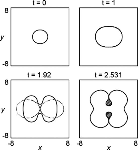
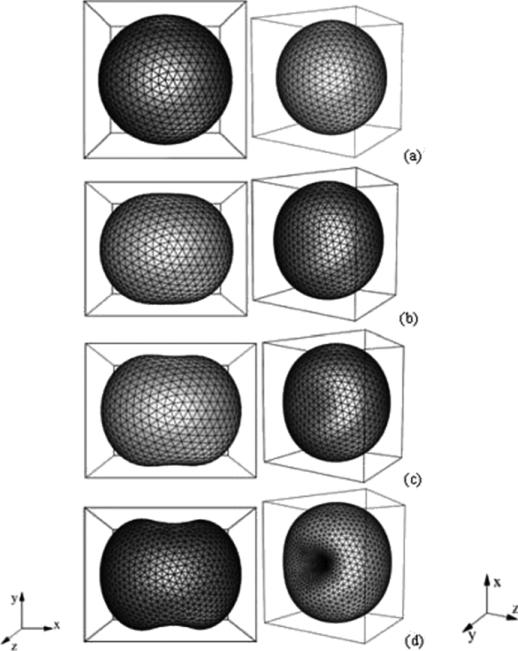
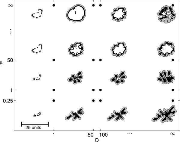
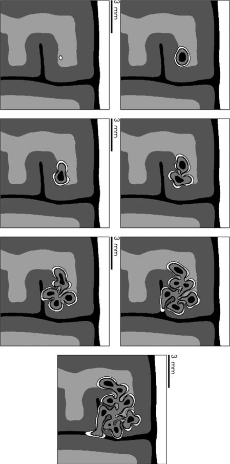
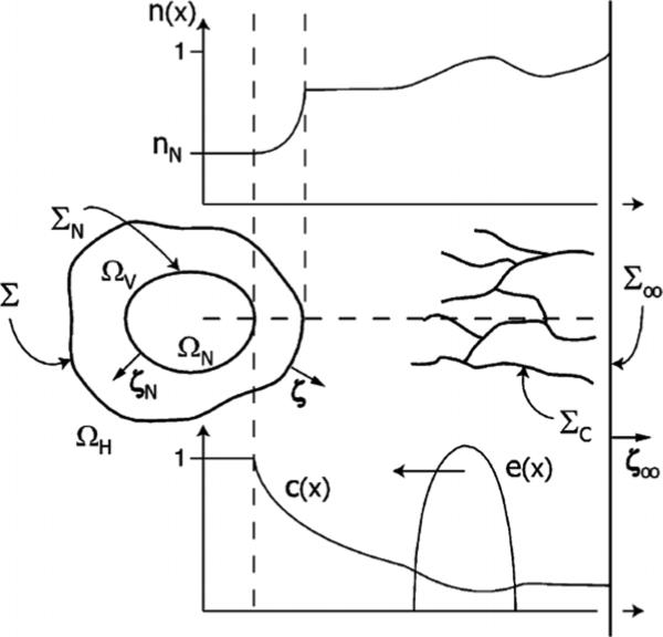
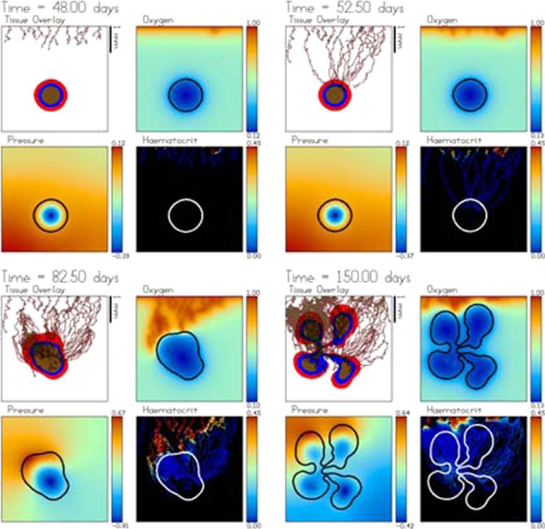
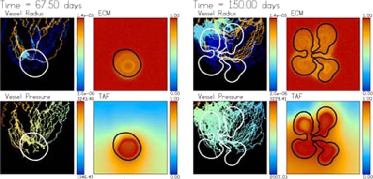
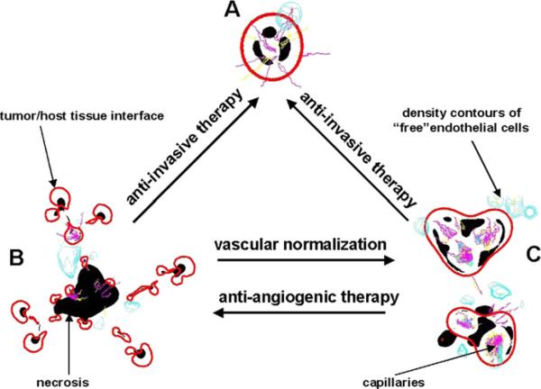
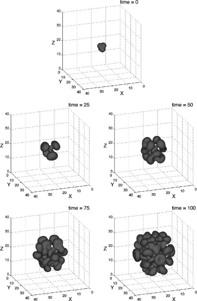
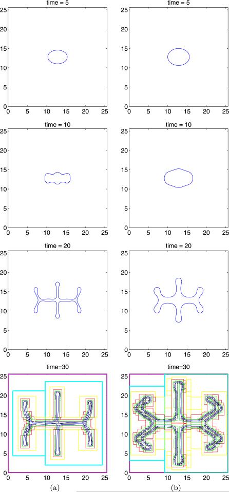
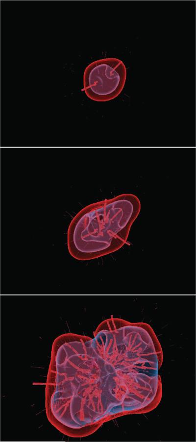
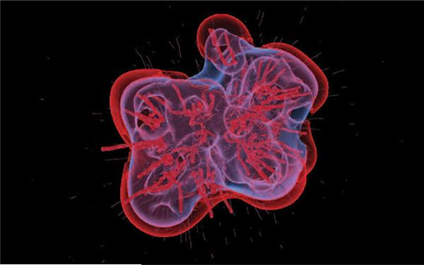
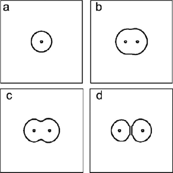
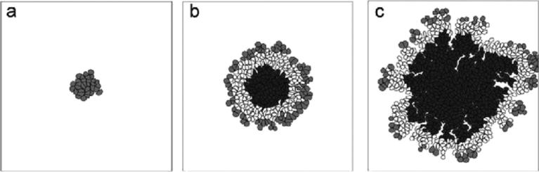
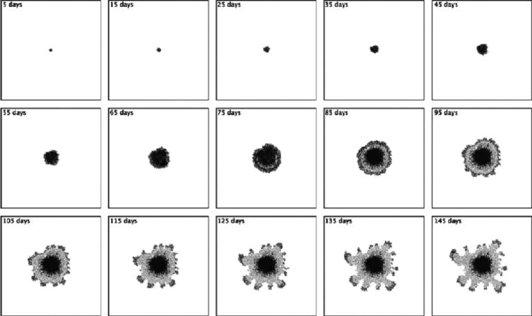
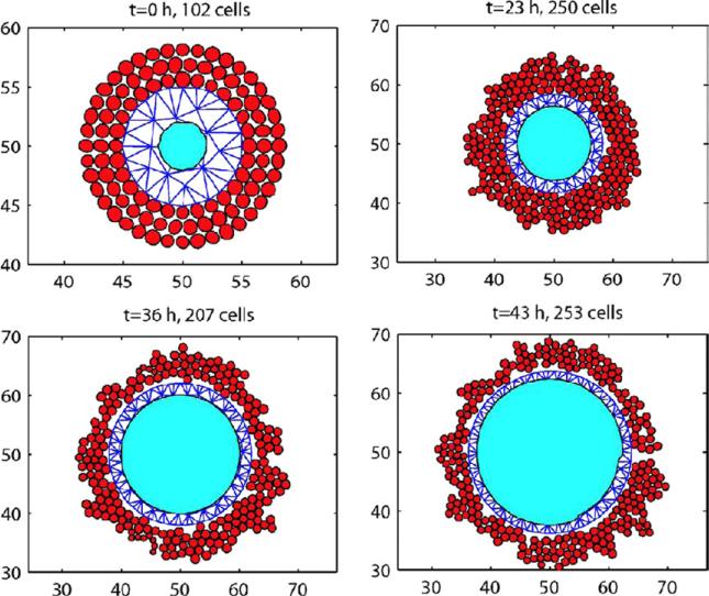
Despite major scientific, medical and technological advances over the last few decades, a cure for cancer remains elusive. The disease initiation is complex, and including initiation and avascular growth, onset of hypoxia and acidosis due to accumulation of cells beyond normal physiological conditions, inducement of angiogenesis from the surrounding vasculature, tumour vascularization and further growth, and invasion of surrounding tissue and metastasis. Although the focus historically has been to study these events through experimental and clinical observations, mathematical modelling and simulation that enable analysis at multiple time and spatial scales have also complemented these efforts. Here, we provide an overview of this multiscale modelling focusing on the growth phase of tumours and bypassing the initial stage of tumourigenesis. While we briefly review discrete modelling, our focus is on the continuum approach. We limit the scope further by considering models of tumour progression that do not distinguish tumour cells by their age. We also do not consider immune system interactions nor do we describe models of therapy. We do discuss hybrid-modelling frameworks, where the tumour tissue is modelled using both discrete (cell-scale) and continuum (tumour-scale) elements, thus connecting the micrometre to the centimetre tumour scale. We review recent examples that incorporate experimental data into model parameters. We show that recent mathematical modelling predicts that transport limitations of cell nutrients, oxygen and growth factors may result in cell death that leads to morphological instability, providing a mechanism for invasion via tumour fingering and fragmentation. These conditions induce selection pressure for cell survivability, and may lead to additional genetic mutations. Mathematical modelling further shows that parameters that control the tumour mass shape also control its ability to invade. Thus, tumour morphology may serve as a predictor of invasiveness and treatment prognosis.

Figure 1

Diagram of a basic non-necrotic tumour. The tumour occupies the volume Ω, Σ is the interface between tumour tissue and health tissue, n is the unit outward normal to Σ.

Figure 2

Analysis of the basic tumour. Top: apoptosis parameter A as a function of unperturbed radius R from condition (19) for self-similar evolution; d = 2 (dashed) and d = 3 (solid); G and l labelled. Asymptotic behaviours are dotted (see [129]). The two solid curves labelled with values of d correspond to stationary radii. Bottom: corresponding growth velocity G⁻¹V for l = 4.

Figure 3

Evaluation of tumour stability. Diagram shows death parameter A versus spheroid radius R (rescaled with diffusion length L). The curves for given values of G are obtained from [194] governing spheroid morphological stability. Experimental conditions for morphologically stable spheroids (shaded area) are enclosed by these and by the horizontal lines delimiting the range of values of A, all estimated by fitting the mathematical model to the in vitro data. The curve ‘stationary radius’ is obtained by setting dR/dt = 0 in equation (1) in [194] governing spheroid radius growth. Three representative stationary spheroid radii are reported on this curve as sampled in vitro. Since this curve crosses and continues beyond the shaded region, most glioma spheroids under these in vitro conditions are marginally stable. Reprinted from Frieboes et al 2006 Cancer Res. 66 1597, with permission from the American Association for Cancer Research.

Figure 4

Analysis of the basic tumour. Left: self-similar shrinkage for R₀ = 4 and δ₀ = 0.2 (t = 0 to 0.96 shown). Right: Unstable shrinkage for R₀ = 4 and δ₀ = 0.4 (t = 0 to 0.99). The solid curves correspond to nonlinear solution and the dashed curves to the linear. In both cases, d = 2, G = 1, l = 5 and the evolution is in the low-vascularization regime. A = A(l,G,R) given in (19) and plotted in figure 2 (top). Reprinted from Cristini et al J. Math. Biol. 46 215. Copyright © 2003 Springer. With kind permission of Springer Science and Business Media.

Figure 5

Evolution of the basic tumour surface in the low-vascularization regime, for d = 2, A = 0.5, G = 20 and initial tumour surface. Dotted lines: solution from linear analysis; solid: solution from a nonlinear calculation with time step Δt = 10⁻³ and a number of marker points N = 1024, reset, after time t = 2.51 to Δt = 10⁻⁴ and N = 2048. Reprinted from Cristini et al J. Math. Biol. 46 202. Copyright © 2003 Springer. With kind = permission of Springer Science and Business Media.

Figure 6

Evolution of the basic tumour surface in the low-vascularization regime, A = 0.5, G = 20 and initial tumour surface as defined in [129]. (a) t = 0, (b) t = 2.21, (c) t = 2.42, (d) t = 2.668. Reprinted with permission from Li et al Discrete Contin. Dyn. Syst.—Ser. B 7 599. Copyright © 2007 American Institute of Mathematical Sciences.

Figure 7

Tumour morphological response to the microenvironment. The external tissue nutrient diffusivity D increases from left to right and the external tissue mobility μ increases from bottom to top. The shape of each tumour is plotted at time T = 20.0. Black regions denote Ω_N where the tumour is necrotic, the grey regions show the viable tumour region Ω_V and the white regions correspond to Ω_H, which consists of the ECM, non-cancerous cells and any other material outside of the tumour. Three major morphologies are observed: fragmenting growth (left), invasive fingering (lower right), and compact/hollow (upper right). All tumours are plotted to the same scale, where the indicated length is 25L ≈ 0.5 cm. Reprinted with permission from Macklin and Lowengrub 2007 J. Theor. Biol. 245 687. Copyright © Elsevier.

Figure 8

Tumour growth in heterogeneous tissue. Simulation from time t = 0.0 days (top left) to t = 60.0 days (bottom right) in 10 day increments. White band on the right of each frame models a rigid material such as the skull; black denotes an incompressible fluid (e.g. cerebrospinal fluid); light and dark grey regions represent tissues of differing biomechanical properties (e.g. white and grey matter). Tumour tissue is shown growing in the middle right with viable (outer layer, white), hypoxic (middle layer, grey), and necrotic (core, black) regions. Reprinted with permission from Macklin and Lowengrub J. Sci. Comput. 35 293–4. Copyright © 2008 Springer (with kind permission of Springer Science and Business Media).

Figure 9

Schematic (not to scale) of a necrotic tumour in transition from avascular to vascular growth. Disjoint regions Ω_H, Ω_V and Ω_N represent healthy tissue viable tumoural tissue and necrotic core domains, respectively. Tumour region is ${\Omega }_{\mathrm{T}}={\Omega }_{\mathrm{V}}\cup {\Omega }_{\mathrm{N}}\cdot {\Sigma }_{\infty }$ is far-field boundary, Σ is tumour interface and Σ_N is necrotic rim. Capillaries are defined on Σ_C. For illustration, nutrient concentration σ(x) (labelled n(x) in the plot), TAF concentration c(x) and endothelial cell density e(x) are plotted along horizontal dashed line. Reprinted with permission from Zheng et al Bull. Math. Biol. 67 215. Copyright © 2005 Springer (with kind permission of Springer Science and Business Media).

Figure 10

Tumour-induced angiogenesis and vascular tumour growth. The vessels respond to the solid pressure generated by the growing tumour. Accordingly, strong oxygen gradients are present that result in strongly heterogeneous tumour cell proliferation and shape instability. The tumour regions (red–proliferating Ω_P, blue–hypoxic/quiescent Ω_H, brown–necrotic Ω_N), the oxygen, mechanical pressure and ECM are shown. The times shown are t = 48 (3 days after angiogenesis is initiated), 52.5, 82.5 and 150 days. Reprinted with permission from Macklin and Lowengrub J. Math. Biol. 58 787. Copyright © 2009 Springer (with kind permission of Springer Science and Business Media).

Figure 11

Dimensional intravascular radius (m) and pressure (Pa) along with the non-dimensional ECM and TAF concentrations from the simulation shown in figure 10. Reprinted with permission from Macklin and Lowengrub J. Math. Biol. 58 788. Copyright © 2009 Springer (with kind permission of Springer Science and Business Media).

Figure 12

Effects of treatment on tumour morphological stability. Solid red: calculated tumour boundary, black: necrosis. The neovasculature (pink) forms from ‘free’ endothelial cells (blue) that chemotax after sprouting from pre-existing vessels (not shown) in outer tissue towards the angiogenic factors in the perinecrotic regions. Reprinted from Cristini et al 2005 Clin. Cancer Res. 11 6772, with permission from the American Association for Cancer Research.

Figure 13

Multiphase model: growth of a two-plus-four mode tumour in 3D with cell adhesion γ = 0. The ϕ_V = 0.5 isosurface is shown. Parameters are the same as for figure 5 in [555]. The model predicts that this tumour morphological instability, which increases the overall surface area to volume ratio, enables the tumour to increase its access to nutrient from the surrounding host vasculature. Reprinted with permission from Frieboes et al J. Theor. Biol. in preparation [192].

Figure 14

Effects of chemotaxis on tumour morphology: evolution of the tumour surface, with $\mathcal{A}=0,\mathcal{D}=1$, ε = 0.005, χ_σ = 5 and the initial tumour surface as (x(α) 12.8, y(α) − 12.8) = (2 + 0.1 cos 2α)(cos α, sin α)). The ϕ = 0.5 contour is shown, where in the interior of the shape ϕ ≈ 1 and in the exterior ϕ ≈ 0. (a) $\mathcal{P}=0.1$; (b) $\mathcal{P}=0.5$. Solid: nonlinear simulation; Dash–dotted: linear results. The last row shows the details of the mesh development. Reprinted with permission from Cristini et al J. Math. Biol. 58 753. Copyright © 2008 Springer (with kind permission of Springer Science and Business Media).

Figure 15

Study of human glioma using a multiscale 3D mixture model [192, 193, 555]. Viable tissue (region between red outer tumour boundary and inner purple boundary), necrosis (region interior to inner purple boundary) and vasculature (thick red lines: mature blood-conducting vessels; thin light red lines: new non-conducting vessels) are shown. The three-month time sequence (top to bottom) shows the effects on the morphology by successive cycles of starvation, neovascularization and vessel co-option [45, 274, 528].

Figure 16

Study of human glioma using a multiscale 3D mixture model [192, 193, 555]. Another view of the simulation from figure 15 at a slightly later time (90 days).

Figure 17

Study of human glioma using a multiscale 3D mixture model [192, 193, 555]. (a): Details of virtual tumour histology showing invasive tumour front (white); locations of blood-conducting new vessels (NV) and non-conducting vessel sprouts (blue dots). Aged vessels in the tumour have thicker walls and are assumed to provide fewer nutrients than the thin-walled vessels at the tumour periphery [400]. (b): H&E stained patient glioblastoma histopathology sections viewed by fluorescence microscopy [193]. Tumour (bottom) is invading normal tissue (top). Note the demarcated margin between tumour and brain parenchyma (middle top), green fluorescent outlines of large, aged vessels deep in the tumour. Bar 100 μm. Reprinted with permission from Frieboes et al NeuroImage 37 S66. Copyright © 2007 Elsevier.

Figure 18

Simulations and experiments of cell protrusions in glioma growing into detached cell clusters and forming separate tumours. Top row: simulation snapshots (time =days) Bottom row: in vitro. Bar: 130 μm. Tumour microsatellites are seen on right. Reprinted from Frieboes et al 2006 Cancer Res. 66 1602, with permission from the American Association for Cancer Research.

Figure 19

Study of ductal carcinoma in situ (DCIS) using the mathematical model of Gatenby and co-workers [230] (colour online). Simulations show potential evolutionary pathways in carcinoma in situ. (a) Simulations start with a single layer of normal epithelial cells (grey cells) on a basement membrane. (b) Initial growth occurred only when mutations produced a hyperproliferative phenotype (pink cells) through mutations (in oncogenes, tumour suppressor genes, etc); growth into the lumen eventually ceased due to hypoxia and acidosis. Without additional cellular evolution, this population remains limited. Additional growth occurred following two possible sequences: (1) heritable changes that upregulate glycolysis. This population with constitutive upregulation (green cells) (c) allows this new population to replace the hyperplastic cells and to extend further into the lumen. However, clonal expansion is eventually limited by acid-mediated toxicity. This promotes evolution of a glycolytic, acid-resistant phenotype (yellow cells) which rapidly replaces all other extant populations in a highly aggressive, infiltrative pattern extending to the basement membrane and farther into the lumen (d). (2) A second pathway begins with development of an acid-resistant population (blue cells). This population expands and replaces many of the hyperplastic population (e) but growth remains limited by hypoxia promoting emergence of a phenotype with upregulated glycolysis and acid resistance (yellow cells) identical to the population in (c). Unlike in (c), this phenotype initially grows into the normoxic region forming nodules of varying size (f ), which eventually coalesce into a pattern essentially identical to the appearance in (d). Reprinted with permission from Gatenby et al Br. J. Cancer 97 649. Copyright © 2007 Nature Publishing Group.

Figure 20

Discrete tumour modelling showing several (eukaryotic) cells from Rejniak [446]. The dots are cell–boundary points which connected by linear springs (thin lines) to model the elastic cell membrane. The interior circles denote cell nucleii. Cell–cell adhesion is also modelled using linear springs between cells (thick lines). Reprinted with permission from Rejniak 2007 J. Theor. Biol. 247 189. Copyright © 2007 Elsevier.

Figure 21

The phases of cell proliferation from Rejniak [446]. (a) The cell begins the mitotic cycle (the interphase); (b) the anaphase—formation of daughter nucleii and an increase in cell volume; (c) the telophase—formation and pinchoff of contractile ring and (d) cytokinesis—the formation of two daughter cells. Reprinted with permission from Rejniak 2007 J. Theor. Biol. 247 190. Copyright © 2007 Elsevier.

Figure 22

Evolution of a 2D avascular tumour from Rejniak [446]. Grey: proliferating cells; white: quiescent cells and black: necrotic cells. Reprinted with permission from Rejniak 2007 J. Theor. Biol. 247 194. Copyright © 2007 Elsevier.

Figure 23

Evolution of a 2D avascular tumour from the discrete model of Anderson [26]. The gradations of colour correspond to different cell phenotypes. The centre region contains necrotic cells. At late times, the outermost region contains the most aggressive cells (highly proliferative, low cell–cell adhesion). Reprinted with permission from Oxford University Press, Anderson 2005 Math. Med. Biol. 22 178.

Figure 24

Hybrid tumour modelling: evolution of a tumour spheroid in the absence of the outer gel from the study by Othmer and co-workers [317]. Necrosis is represented by the inner (white) region; it is enclosed by the continuum quiescent region and the outer cell-based region (space unit = 10 μm). Reprinted with permission from Kim et al Math. Models Methods Appl. Sci. 17 1790. Copyright © (2007) World Scientific.

Figure 25

Evolution of a vascularized tumour using a hybrid continuum–discrete model for tumour cells. Discrete cells (blue) dots are released from hypoxic regions of the continuous tumour regions (grey). Discrete cells are converted back to continuum volume fractions when their density is sufficiently large. Vessel sprouts (yellow) and newly formed vessels releasing oxygen (dark brown) are shown.

References

1. Abbott RG, Forrest S, Pienta KJ. Simulating the hallmarks of cancer. Art. Life. 2006;12:617–34. - PubMed
1. Abia LM, Angulo O, Lopez-Marcos JC. Age-structured population models and their numerical solution. Ecol. Modelling. 2005;188:112–36.
1. Adam JA. A simplified mathematical model of tumor growth. Math. Biosci. 1986;81:229–44.
1. Adam JA. A mathematical model of tumor growth: II. Effects of geometry and spatial nonuniformity on stability. Math. Biosci. 1987;86:183–211.
1. Adam JA. A mathematical model of tumor growth: III. Comparison with experiment. Math. Biosci. 1987;86:213–27.