. 2011 Apr;30(2):471-87.
doi: 10.1007/s10827-010-0272-1. Epub 2010 Sep 1.

A continuous mapping of sleep states through association of EEG with a mesoscale cortical model

Affiliations

A continuous mapping of sleep states through association of EEG with a mesoscale cortical model

Beth A Lopour et al. J Comput Neurosci. 2011 Apr.

Abstract

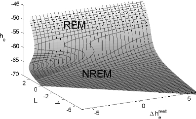
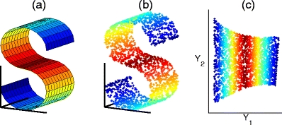
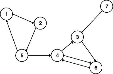
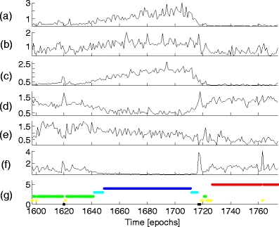
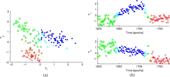
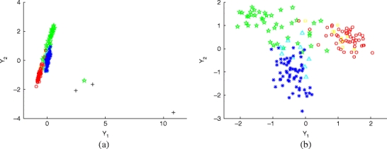
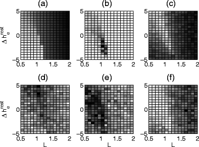
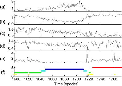
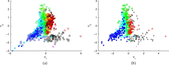
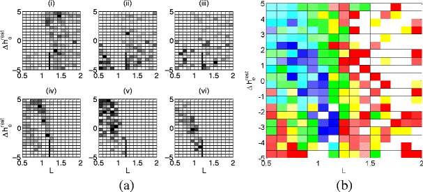
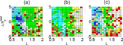
Here we show that a mathematical model of the human sleep cycle can be used to obtain a detailed description of electroencephalogram (EEG) sleep stages, and we discuss how this analysis may aid in the prediction and prevention of seizures during sleep. The association between EEG data and the cortical model is found via locally linear embedding (LLE), a method of dimensionality reduction. We first show that LLE can distinguish between traditional sleep stages when applied to EEG data. It reliably separates REM and non-REM sleep and maps the EEG data to a low-dimensional output space where the sleep state changes smoothly over time. We also incorporate the concept of strongly connected components and use this as a method of automatic outlier rejection for EEG data. Then, by using LLE on a hybrid data set containing both sleep EEG and signals generated from the mesoscale cortical model, we quantify the relationship between the data and the mathematical model. This enables us to take any sample of sleep EEG data and associate it with a position among the continuous range of sleep states provided by the model; we can thus infer a trajectory of states as the subject sleeps. Lastly, we show that this method gives consistent results for various subjects over a full night of sleep and can be done in real time.


Figures

Fig. 1
Fig. 1
The manifold of steady states in h e from the mesoscale cortical model, hereafter referred to as the “sleep manifold.” The parameters L and formula image represent the actions of adenosine and acetylcholine, neuromodulators that vary over the course of the human sleep cycle. The manifold has two stable solutions on its left side; a jump from the bottom solution to the top solution represents the fast transition between NREM and REM sleep. However, the slow transition from REM to NREM occurs smoothly down the right side of the manifold, where there is only one set of solutions
Fig. 2
Fig. 2
A simple example of LLE, where three dimensions are reduced to two. (a) The underlying manifold, which lives in 3D space but has only two dimensions. In a typical LLE problem, the shape of this manifold is unknown and has too many dimensions to visualize easily. (b) A sampling of points from the manifold, which serves as the input to the LLE algorithm. (c) The result of applying LLE to the data set in (b). Note that in the Y 1 − Y 2 output space, the manifold has been flattened to reveal its two principal dimensions. This figure was generated using the “scurve.m” code from the LLE website (Roweis and Saul 2009)
Fig. 3
Fig. 3
An example of a directed graph generated by nearest neighbor associations. Here point 2 is a neighbor of point 1, point 3 is a neighbor of point 7, etc. In this case, the directed graph forms two strongly connected components: points 1, 2, 5, and points 3, 4, 6. In analyzing this data set, we would use LLE separately on each of these components and would remove point 7, which is not strongly connected to any other point
Fig. 4
Fig. 4
Scaled features of EEG data set sc4002e0, as described in Section 4.2. The subfigures show power in the (a) delta and (b) theta bands, (c) variance, (d) spindle score, (e) maximum height of the power spectrum in the alpha band after subtraction of a linear estimate, and (f) high power fraction. Figure (g) shows the hypnogram of the EEG data, where the number and color indicate the sleep stage: awake (0, black), stage 1 (1, yellow), stage 2 (2, green), stage 3 (3, cyan), stage 4 (4, blue), and REM (5, red). The features were calculated for the data from epochs 1,597–1,774 in 30-second windows with no overlap
Fig. 5
Fig. 5
(a) Results of applying LLE to EEG data using the six features in Fig. 4. The features were calculated for 30-second non-overlapping windows of data and the resulting 6-dimensional points were embedded in 2D space using LLE with k = 13; therefore, each point in this figure represents 30 s of EEG that has been characterized by the six features. The color and shape indicate sleep stage based on manual scoring: awake (black +), stage 1 (yellow formula image), stage 2 (green ⋆), stage 3 (cyan ∆), stage 4 (blue ∗), and REM (red ∘). (b) LLE output dimensions Y 1 and Y 2 versus time, for the results shown in (a). This demonstrates that LLE provides a low-dimensional output where the sleep state changes smoothly over time
Fig. 6
Fig. 6
LLE results on sleep EEG data before (a) and after (b) removal of eight weakly connected points. The six features were power in the delta, theta, and gamma bands, total power, maximum height of PSD above a linear estimate in the alpha band, and low power fraction, and we used k = 13. As before, the color and symbol indicate sleep stage: awake (black +), stage 1 (yellow formula image), stage 2 (green ⋆), stage 3 (cyan ∆), stage 4 (blue ∗), and REM (red ∘). Note the dramatic improvement in separation between sleep stages when LLE is done on only one strongly connected component in (b)
Fig. 7
Fig. 7
Variation of five features as the surface of the sleep manifold is traversed in L-formula image space. Each feature has been scaled by its RMS value and depicted in grayscale, with white indicating the lowest values and black representing the highest values. (a) The steady state values of h e from the sleep manifold in Fig. 1. The black points represent the upper REM branch, the white points represent NREM, and the fold is located at roughly L = 1.2. The other subfigures show (b) power in the delta band, (c) permutation entropy, (d) maximum height of PSD above a linear estimate in the alpha band, (e) low power fraction, and (f) high power fraction. These five features use α as defined in Eq. (15). They show that the representation of REM and NREM in the model is consistent with the characteristics of sleep EEG
Fig. 8
Fig. 8
Variation of the features from Fig. 7 when they are applied to sleep EEG data, rather than model data. The sample of EEG data was taken from sc4002e0, and each feature has been scaled by its RMS value. The subfigures show (a) power in the delta band, (b) permutation entropy, (c) maximum height of PSD above a linear estimate in the alpha band, (d) low power fraction, (e) high power fraction, and (f) hypnogram of the EEG data. The colors and numbering for the hypnogram are the same as those used for Fig. 4. Note that the values of these features (relative to sleep stage) are consistent with the model results in Fig. 7
Fig. 9
Fig. 9
(a) LLE results for a hybrid data set containing both sleep EEG data and numerical solutions of the cortical model. We used the five features from Fig. 7 and set k = 14. The rings represent EEG data and are colored by sleep stage. While the analysis included 1,200 windows of EEG data, only 500 are displayed here for clarity. The solid dots represent data from the model; they are colored based on the mean value of h e at that point, where red represents the highest (REM) values, and dark blue marks the lowest (NREM) values. Note that the data and model points overlap in the output space and that the arrangement of sleep stages is very similar. (b) LLE results showing the EEG data only, using the same colors and symbols as Fig. 6. This allows us to see that the data has been roughly separated by sleep stage
Fig. 10
Fig. 10
Association between EEG data set sc4002e0 and the sleep manifold. Each picture shows the sleep manifold in L-formula image space, with a heavy black line to indicate the location of the fold. (a) Histograms of nearest neighbors for (i) waking, (ii) REM, (iii) stage 1, (iv) stage 2, (v) stage 3, and (vi) stage 4 sleep. The shading of each square indicates the number of times that location on the sleep manifold was a nearest neighbor of EEG data in that stage. For example, (vi) shows that stage 4 sleep most often associates itself with the lower NREM branch of solutions leading up to the fold. (b) A composite picture of the results in (a), where each location is colored based on the sleep stage with the most neighbors at that point, relative to the total number of neighbors associated with that stage. Again, we use stage 1 (yellow), stage 2 (green), stage 3 (cyan), stage 4 (blue), and REM (red). The intensity of color is scaled based on the percentage of neighbors that come from that stage; the more saturated the color, the greater the percentage. Waking points were excluded
Fig. 11
Fig. 11
Composite plots for EEG data sets (a) sc4012e0, (b) sc4102e0, and (c) sc4112e0, when they are projected onto the LLE results from Fig. 6(b), as described in Section 5.4. These pictures are analogous to Fig. 10(b) and use the same color scheme. Note that the results are consistent with those for sc4002e0 in Fig. 10(b); over various subjects, the sleep stages are generally associated with the same positions on the sleep manifold
Fig. 12
Fig. 12
Combined association between all four EEG data sets and the sleep manifold. The data set sc4002e0 was directly compared to the cortical model using LLE, and the remaining three data sets were projected onto those results as described in Section 5.4. (a) Total histograms of nearest neighbors, separated by sleep stage; these were calculated by summing the histograms from all four EEG data sets. The pictures show awake, REM, and stages 1–4 in (i) through (vi), respectively. (b) The total composite picture for all four data sets. This was generated from the histogram data in (a) and is analogous to Figs. 10(b) and 11. Again, this is consistent with previous results and shows the regions of the sleep manifold most closely associated with each sleep stage

Similar articles

Cited by

References

    1. Ataee, P., Yazdani, A., Setarehdan, S. K., & Noubari, H. A. (2007). Manifold learning applied on EEG signal of the epileptic patients for detection of normal and pre-seizure states. In Proceedings of the 29th Annual International Conference of the IEEE EMBS (pp. 5489–5492). - PubMed
    1. Bojak, I., & Liley, D. T. (2005). Modeling the effects of anesthesia on the electroencephalogram. Physical Review E, 71(041902). - PubMed
    1. Corsi-Cabrera M, Guevara MA, Río-Portilla YD, Arce C, Villanueva-Hernández Y. EEG bands during wakefulness, slow-wave and paradoxical sleep as a result of principal component analysis in man. SLEEP. 2000;23(6):1–7. - PubMed
    1. Fuller P, Gooley J, Saper C. Neurobiology of the sleep-wake cycle: Sleep architecture, circadian regulation, and regulatory feedback. Journal of Biological Rhythms. 2006;21(6):482–493. doi: 10.1177/0748730406294627. - DOI - PubMed
    1. Fuller P, Saper C, Lu J. The pontine rem switch: Past and present. Journal of Physiology. 2007;584(3):735–741. doi: 10.1113/jphysiol.2007.140160. - DOI - PMC - PubMed

Publication types