Classic and contemporary approaches to modeling biochemical reactions

Abstract

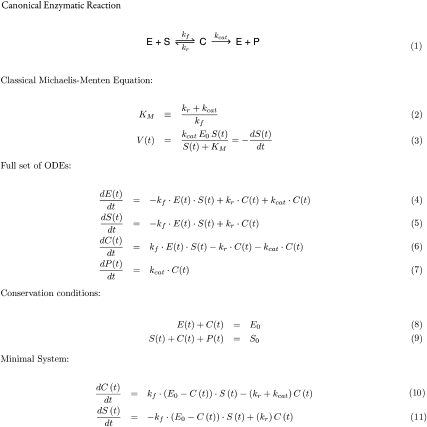
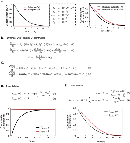
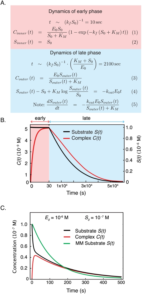
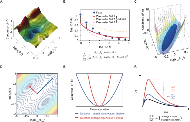
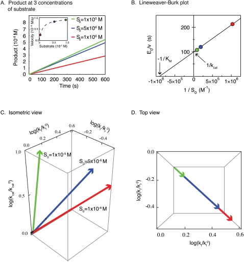
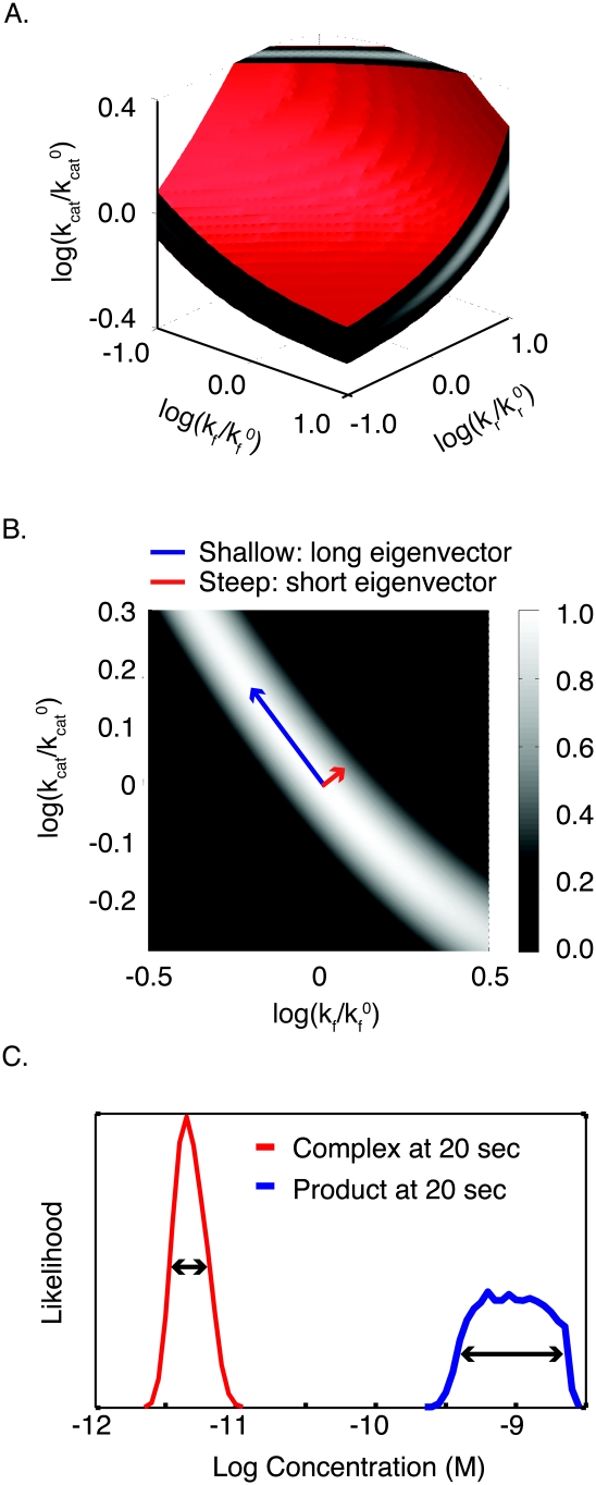
Recent interest in modeling biochemical networks raises questions about the relationship between often complex mathematical models and familiar arithmetic concepts from classical enzymology, and also about connections between modeling and experimental data. This review addresses both topics by familiarizing readers with key concepts (and terminology) in the construction, validation, and application of deterministic biochemical models, with particular emphasis on a simple enzyme-catalyzed reaction. Networks of coupled ordinary differential equations (ODEs) are the natural language for describing enzyme kinetics in a mass action approximation. We illustrate this point by showing how the familiar Briggs-Haldane formulation of Michaelis-Menten kinetics derives from the outer (or quasi-steady-state) solution of a dynamical system of ODEs describing a simple reaction under special conditions. We discuss how parameters in the Michaelis-Menten approximation and in the underlying ODE network can be estimated from experimental data, with a special emphasis on the origins of uncertainty. Finally, we extrapolate from a simple reaction to complex models of multiprotein biochemical networks. The concepts described in this review, hitherto of interest primarily to practitioners, are likely to become important for a much broader community of cellular and molecular biologists attempting to understand the promise and challenges of "systems biology" as applied to biochemical mechanisms.

Figure 1.

The canonical enzymatic reaction (Eq. 1) analyzed by Michaelis-Menten, and the resulting equations defining K_M (Michaelis constant) and V(t) (velocity) (Eqs. 2,3). (Eqs. 4–7) The same enzymatic reaction described using a coupled set of four ODEs, defining changes in the concentration of enzyme, substrate, complex, and product over time. Using conservation conditions (Eqs. 8,9), the set of four ODEs can be reduced to two equations, describing the change over time of complex and substrate (Eqs. 10,11).

Figure 2.

Nondimensionalization and singular perturbation analysis of a simple enzymatic reaction, fulfilling the Michaelis-Menten conditions. (A, left) The trajectories for concentrations of substrate (black) and complex (red) over time. (Right) The rescaled graph using nondimensionalized parameters illustrates the behavior of both species on a common axis, and suggests the existence of two separable time scales. (B) The dynamic ODEs after rescaling for concentration. (C) The same equations as in B, with a specific set of parameters drawn from A. The difference of approximately two orders of magnitude in the nondimensionalized reaction rate constants indicates two distinct and therefore separable time scales. (D) The inner solution of the nondimensionalized dynamical system showing the early, fast phase, during which complex formation rises exponentially (red), while the substrate concentration remains constant (black). (E) The outer solution of the nondimensionalized dynamical system showing the coupled decay of complex (red) and substrate (black), with complex in rapid pseudoequilibration with falling substrate.

Figure 3.

Singular perturbation analysis of the classical enzyme reaction. (A) The equation set describing the dynamics of the early (fast; pink) and late (slow; blue) phase of the reaction. The time scale of each of the phases is indicated. (B) Nondimensionalized changes in complex (red) and substrate (black) smoothly joined following singular perturbation analysis for the early (pink) and late (blue) phase of the reaction. (C) Example of a reaction system that can be analyzed by singular perturbation methods but that does not fulfill requirements of the classical Michaelis-Menten approximation. Complex (red) and substrate (black) exhibit a fast and slow phase. The Michaelis-Menten approximation of substrate (green) shows substantial deviation from the true dynamics.

Figure 4.

Parameter values for dynamical systems described by ODEs can be estimated from data using an objective function. (A) In the objective function, each unknown parameter of the ODE system corresponds to a dimension. The surface of the objective function resembles an energy landscape, with the altitude at each point denoting the goodness of fit of a specific set of parameters to data. Here, a three-dimensional slice through a complex objective function (corresponding to two parameters) shows numerous steep inclines/declines, local maxima/minima, and large areas where the objective function is independent of the two parameters displayed. (B) The deviation between points of synthetic data and model trajectories can be measured and used to evaluate the parameters. The effect of assuming perfect data means that there is a well-defined minimum that is the “true” parameter set, while the assumption of a variance means that the χ² landscape has realistic values for its peaks and valleys. (C) The approximated surface of a particular valley in the complex landscape is shown in blue. (D) The curvature of the approximated surface area can be calculated as the second term of the Taylor expansion of the objective function, the Hessian. The eigenvectors of the Hessian represent the short and long axes of the paraboloid, and generally do not point in the direction of any single parameter. (E) Short eigenvectors indicate the direction of a steep parabola (large eigenvalue; red), and long eigenvectors indicate the direction of a shallow parabola (small eigenvalue; blue). (F) Moving in the direction of either eigenvector in parameter space has different consequences for model trajectories. Moving along a steep eigenvector of a Hessian leads to significant changes in the trajectory (red), while moving along the shallow eigenvector leads to only minor changes (blue), corresponding respectively to large and small changes in the values of the objective function.

Figure 5.

The Michaelis-Menten approximation of a classical enzymatic reaction and the connection to parameter identifiability. (A) In typical experiments, V_max (enzyme velocity) can be determined for various concentrations of substrate. (B) The reciprocal plots of the measured values can be plotted to determine the Michaelis constant (K_M) and the catalytic constant (k_cat). (C) Measuring enzyme velocity for three substrate concentrations projects individual vectors in the three-dimensional parameter space. (D) While altering the substrate concentration allows for the determination of k_cat, the ratio of the reverse rate constant to the forward rate constant (k_r/k_f) remains unchanged. Thus, only K_M can be determined, leaving the k_f and k_r reaction rate constants undetermined.

Figure 6.

The likelihood function ascribes the likelihood of correctness to parameter sets based on how well they explain the observed data. (A) The surface plot of the χ² error function of the classical enzyme reaction in parameter space. The likelihood of a given parameter set is given by the brightness (white being most likely), while red denotes a cutoff boundary. (B) A two-dimensional slice through the χ² function shows that the likelihood of one parameter (e.g., k_f) is dependent on another parameter (e.g., k_cat). The region of high likelihood (white) corresponds directly to the shallow direction of a Hessian (i.e., all yielding similarly low values of the objective function). (C) Sampling of parameter sets using the likelihood function can be used to make probabilistic predictions of product (blue) and complex (red) formation at 20 sec after the start of the reaction. While individual parameters of the reaction rate constants remain nonidentifiable, specific and unique predictions can be made.

References

1. Agirrezabala X, Lei J, Brunelle JL, Ortiz-Meoz RF, Green R, Frank J 2008. Visualization of the hybrid state of tRNA binding promoted by spontaneous ratcheting of the ribosome. Mol Cell 32: 190–197 - PMC - PubMed
1. Albeck JG, Burke JM, Spencer SL, Lauffenburger DA, Sorger PK 2008. Modeling a snap-action, variable-delay switch controlling extrinsic cell death. PLoS Biol 6: 2831–2852 - PMC - PubMed
1. Atkins GL, Nimmo IA 1975. A comparison of seven methods for fitting the Michaelis-Menten equation. Biochem J 149: 775–777 - PMC - PubMed
1. Atkinson AC, Donev AN 1992. Optimum experimental designs. Clarendon Press, Oxford
1. Bandara S, Schloder JP, Eils R, Bock HG, Meyer T 2009. Optimal experimental design for parameter estimation of a cell signaling model. PLoS Comput Biol 5: e1000558 doi: 10.1371/journal.pcbi.1000558 - PMC - PubMed
Publication types