A framework for feature selection in clustering

Abstract

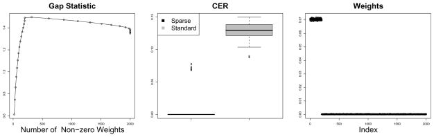
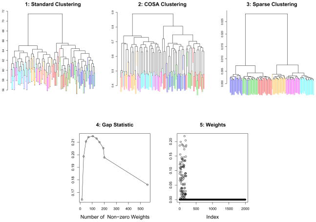
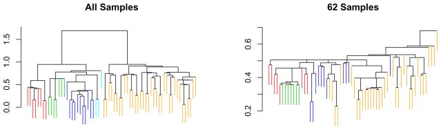
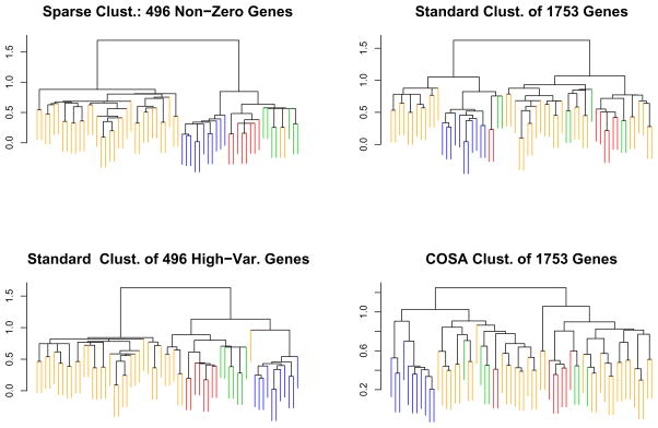
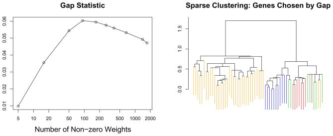
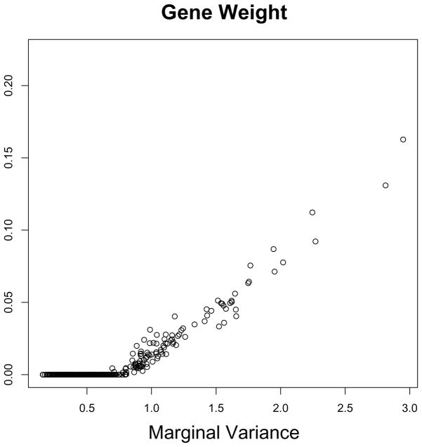
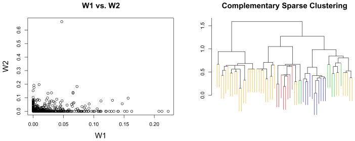
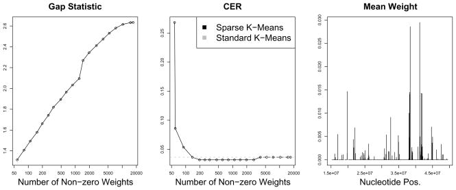
We consider the problem of clustering observations using a potentially large set of features. One might expect that the true underlying clusters present in the data differ only with respect to a small fraction of the features, and will be missed if one clusters the observations using the full set of features. We propose a novel framework for sparse clustering, in which one clusters the observations using an adaptively chosen subset of the features. The method uses a lasso-type penalty to select the features. We use this framework to develop simple methods for sparse K-means and sparse hierarchical clustering. A single criterion governs both the selection of the features and the resulting clusters. These approaches are demonstrated on simulated data and on genomic data sets.

Figure 1

In a two-dimensional example, two classes differ only with respect to the first feature. Sparse 2-means clustering selects only the first feature, and therefore yields a superior result.

Figure 2

Sparse and standard 6-means clustering are applied to a simulated 6-class example. Left: The gap statistics obtained using the sparse 6-means tuning parameter selection method, as a function of the number of features with non-zero weights, averaged over 10 simulated data sets. Center: Boxplots of the CERs obtained using sparse and standard 6-means clustering on 100 simulated data sets. Right: The weights obtained using sparse 6-means clustering, averaged over 100 simulated data sets.

Figure 3

Standard hierarchical clustering, COSA, and sparse hierarchical clustering with complete linkage were performed on simulated 6-class data. 1, 2, 3: The color of each leaf indicates its class identity. CERs were computed by cutting each dendrogram at the height that results in 6 clusters: standard, COSA, and sparse clustering yielded CERs of 0.169, 0.160, and 0.0254. 4: The gap statistics obtained for sparse hierarchical clustering, as a function of the number of features included for each value of the tuning parameter. 5: The w obtained using sparse hierarchical clustering; note that the six classes differ with respect to the first 200 features.

Figure 4

Using the intrinsic gene set, hierarchical clustering was performed on all 65 observations (left panel) and on only the 62 observations that were assigned to one of the four classes (right panel). Note that the classes identified using all 65 observations are largely lost in the dendrogram obtained using just 62 observations. The four classes are basal-like (red), Erb-B2 (green), normal breast-like (blue), and ER+ (orange). In the left-hand panel, observations that do not belong to any class are shown in light blue.

Figure 5

Four hierarchical clustering methods were used to cluster the 62 observations that were assigned to one of four classes in Perou et al. (2000). Sparse clustering results in the best separation between the four classes. The color coding is as in Figure 4.

Figure 6

The gap statistic was used to determine the optimal value of the tuning parameter for sparse hierarchical clustering. Left: The largest value of the gap statistic corresponds to 93 genes with non-zero weights. Right: The dendrogram corresponding to 93 non-zero weights. The color coding is as in Figure 4.

Figure 7

For each gene, the sparse clustering weight is plotted against the marginal variance.

Figure 8

Complementary sparse clustering was performed. Tuning parameters for the initial and complementary clusterings were selected to yield 496 genes with non-zero weights. Left: A plot of w₁ against w₂. Right: The dendrogram for complementary sparse clustering. The color coding is as in Figure 4.

Figure 9

Left: The gap statistics obtained as a function of the number of SNPs with non-zero weights. Center: The CERs obtained using sparse and standard 3-means clustering, for a range of values of the tuning parameter. Right: Sparse clustering was performed using the tuning parameter that yields 198 non-zero SNPs (this is the smallest number of SNPs that resulted in minimal CER in the center panel). Chromosome 22 was split into 500 segments of equal length. The average weights of the SNPs in each segment are shown, as a function of the nucleotide position of the segments.

References

1. Boyd S, Vandenberghe L. Convex Optimization. Cambridge University Press; 2004.
1. Chang W-C. On using principal components before separating a mixture of two multivariate normal distributions. Journal of the Royal Statistical Society, Series C (Applied Statistics) 1983;32:267–275.
1. Chipman H, Tibshirani R. Hybrid hierarchical clustering with applications to microarray data. Biostatistics. 2005;7:286–301. - PubMed
1. Dempster A, Laird N, Rubin D. Maximum likelihood from incomplete data via the EM algorithm (with discussion) J R Statist Soc B. 1977;39:1–38.
1. Eisen M, Spellman P, Brown P, Botstein D. Cluster analysis and display of genome-wide expression patterns. Proc Natl Acad Sci, USA. 1998;95:14863–14868. - PMC - PubMed
Publication types
LinkOut - more resources