Imaging Brain Dynamics Using Independent Component Analysis

Abstract

The analysis of electroencephalographic (EEG) and magnetoencephalographic (MEG) recordings is important both for basic brain research and for medical diagnosis and treatment. Independent component analysis (ICA) is an effective method for removing artifacts and separating sources of the brain signals from these recordings. A similar approach is proving useful for analyzing functional magnetic resonance brain imaging (fMRI) data. In this paper, we outline the assumptions underlying ICA and demonstrate its application to a variety of electrical and hemodynamic recordings from the human brain.

Fig. 1

The difference between PCA and ICA on a nonorthogonal mixture of two distributions that are independent and highly sparse (peaked with long tails). An example of a sparse distribution is the Laplacian: p(x) = ke^|−x|. PCA, looking for orthogonal axes ranked in terms of maximum variance, completely misses the structure of the data. Although these distributions may look strange, they are quite common in natural data.

Fig. 2

Optimal information flow in sigmoidal neurons. (left) Input x raving probability density function p(x), n this case a Gaussian, is passed through a nonlinear function g(x). The information in the resulting density, p(x) depends on matching the mean and variance of x to the threshold, w₀, and slope, w, of g(x) (Nicol Schraudolph, personal communication). (right) p(y) is plotted for different values of the weight w. The optimal weight, w_opt transmits most information (from [2] by permission.)

Fig. 3

A selection of 144 basis functions (columns of W⁻¹) obtained from training on patches of 12-by-12 pixels from pictures of natural scenes.

Fig. 4

(a) Grand mean evoked response to detected target stimuli in the detection task (average of responses from ten subjects and five attended locations). Response waveform at all 29 scalp channels and two EOG channels are plotted on a common axis. Topographic plots of the scalp distribution of the response at four indicated latencies show that the LPC topography is labile, presumably reflecting the summation at the electrodes of potentials generated by temporally overlapping activations in several brain areas each having broad but topographically fixed projections to the scalp. All scalp maps shown individually scaled to increase color contrast, with polarities at their maximum projection as indicated in the color bar. (b) Activation time courses and scalp maps of the four LPC components produced by Infomax ICA applied to 75 1-s grand-mean (10-Ss) ERPs from both tasks. Map scaling as in (a). The thick dotted line (left) indicates stimulus onset. Mean subject-median response times (RTs) in the Detection task (red) and Discrimination task (blue) are indicated by solid vertical bars. Three independent components (P3f, P3b, Pmp) accounted for 95%–98% of response variance in both tasks. In both tasks, median RT coincided with Pmp onset. The faint vertical dotted line near 250 ms shows that the P3f time courses for targets and “nogo” nontargets (presented in the target location) just at the onset of the left-sided Pnt component, which was active only in this condition. (c) Envelopes of the scalp projections of maximally independent component P3f, (red filled) superimposed on the mean response envelopes (black outlines) for all 5 × 5 response conditions of the Detection task. (d) The top panels show the grand mean target response at two scalp channels, Fz and Pz (thick traces), and the projections of the two largest ICA components, P3b and Pmp, to the same channels (thin traces). The central panel shows a scatter plot of ten average target ERPs at the two electrodes. The data contain two strongly radial (and, therefore, spatially fixed) features. The dashed lines (middle panel) show the directions associated with components P3b and Pmp in these data, as determined by the relative projection strengths of each component to these two scalp channels (shown below as black dots on the component scalp maps). The degree of data entropy attained by ICA training is illustrated by the (center right) plot insert, which shows the (31-channel) scatter-plotted data after logistic transformation and rotation to the two component axes (from [25] by permission).

Fig. 5

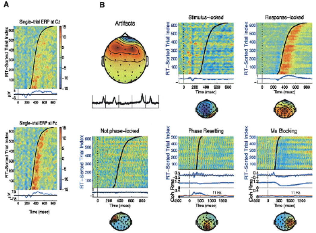
ERP-image plots of target response data from a visual selective attention experiment and various independent component categories. (a) Single-trial ERPs recorded at a central (Cz) and a parietal electrode (Pz) from an autistic subject and timelocked to onsets of visual target stimuli (left thin vertical line) with superimposed subject response times (RT). (b) Single-trial activations of sample independent components accounting for (clockwise) eye blink artifacts, stimulus-locked and response-locked ERP components, response-blocked oscillatory mu, stimulus phase-reset alpha, and nonphase locked activities.

Fig. 6

ERP-image plot of single-trial activations of one alpha component from the selective visual attention experiment described in Section IV. Top image: Single-trial potentials, color coded (scale: red positive, green zero and blue negative). Blue traces below image: (top trace) averaged evoked response activity of this component, showing “alpha ringing.” Units: proportional to µV. (middle trace) Time course of rms amplitude of this component at its peak frequency, 10 Hz. Units: relative to log₁₀ (µV²). (bottom trace) Time course of inter-trial coherence at 10 Hz. (thick), plus the bootstrap (p = 0.02) significance threshold (thin). Intertrial coherence measures the tendency for phase values at a given time and frequency to be fixed across trials. Bottom left: Mean power spectral density of the component activity (units, relative decibels). Bottom right: scalp map showing the interpolated projection of the component to the scalp electrodes.

Fig. 7

(a) An fMRI experiment was performed in which the subject was instructed to perform 15-s blocks of alternating right wrist supination and pronation, alternating with 15-s rest blocks. The movement periods where alternately self-paced or were visually cued by a movie showing a moving hand. (b) ICA analysis of the experiment detected a spatially independent component that was active during both types of motor periods but not during rest. The spatial distribution of this component (threshold, z ≥ 2) was in the contralateral primary motor area and ipsilateral cerebellum. (The radiographic convention is used here, the right side of the image corresponding to the left side of the brain and vice versa) (from McKeown, et al., manuscript in preparation). (c) A similar fMRI experiment was performed in which the subject supinated/pronated both wrists simultaneously. Here, ICA detected a component that was more active during self-paced movements than during either visually cued movement or rest periods. The midline region depicted threshold, z ≥ 2 is consistent with animal studies showing relative activation of homologous areas during self-paced but not visually cued tasks. (e.g. [69]).

References

-
- Herault J, Jutten C. Space or time adaptive signal processing by neural network models; presented at the Neural Networks for Computing: AIP Conf; 1986.
- Jutten C, Herault J. Blind separation of sources I. An adaptive algorithm based on neuromimetic architecture. Signal Process. 1991;vol. 24:1–10.
- Pham DT, Garat P, Jutten C. Separation of a mixture of independent sources through a maximum likelihood approach. presented at the Proc. EUSIPCO. 1992
- Comon P. Independent component analysis, a new concept? Signal Process. 1994;vol. 36:287–314.
- Cichocki A, Unbehauen R, Rummert E. Robust learning algorithm for blind separation of signals. Electron. Lett. 1994;vol. 30:1386–1387.
Grants and funding
LinkOut - more resources
Full Text Sources
Other Literature Sources
Miscellaneous