A network of spiking neurons that can represent interval timing: mean field analysis

Abstract

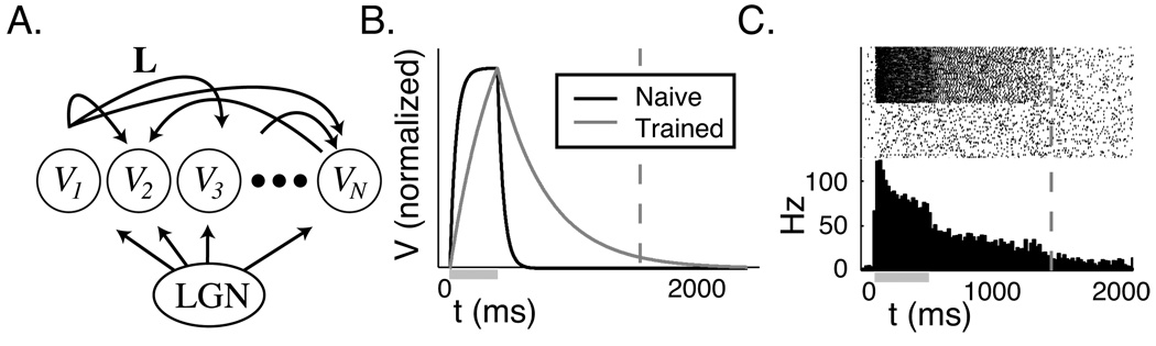
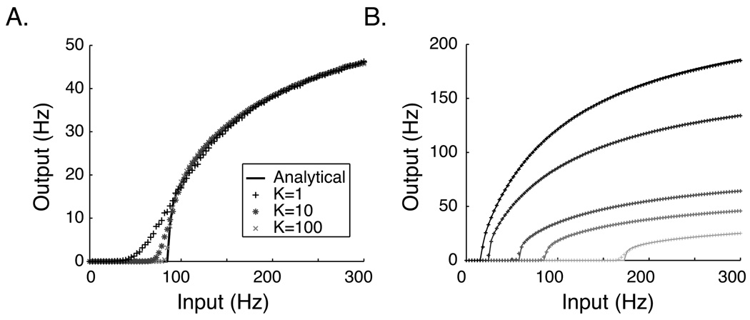
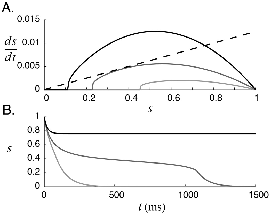
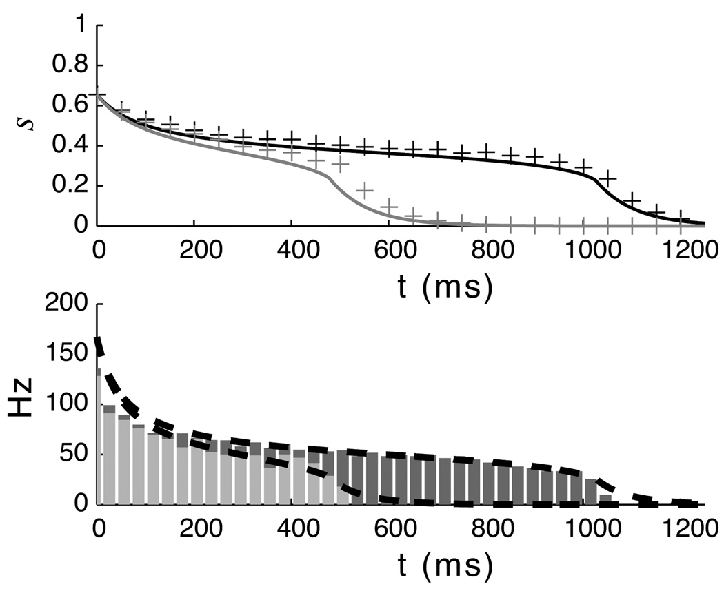
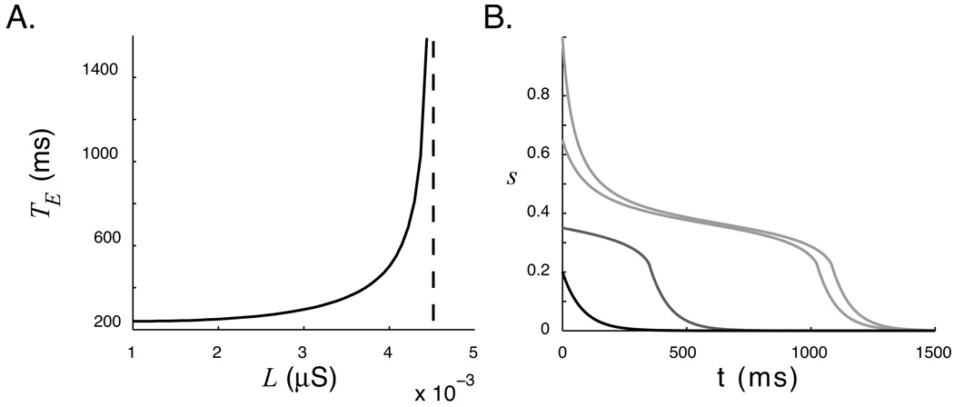
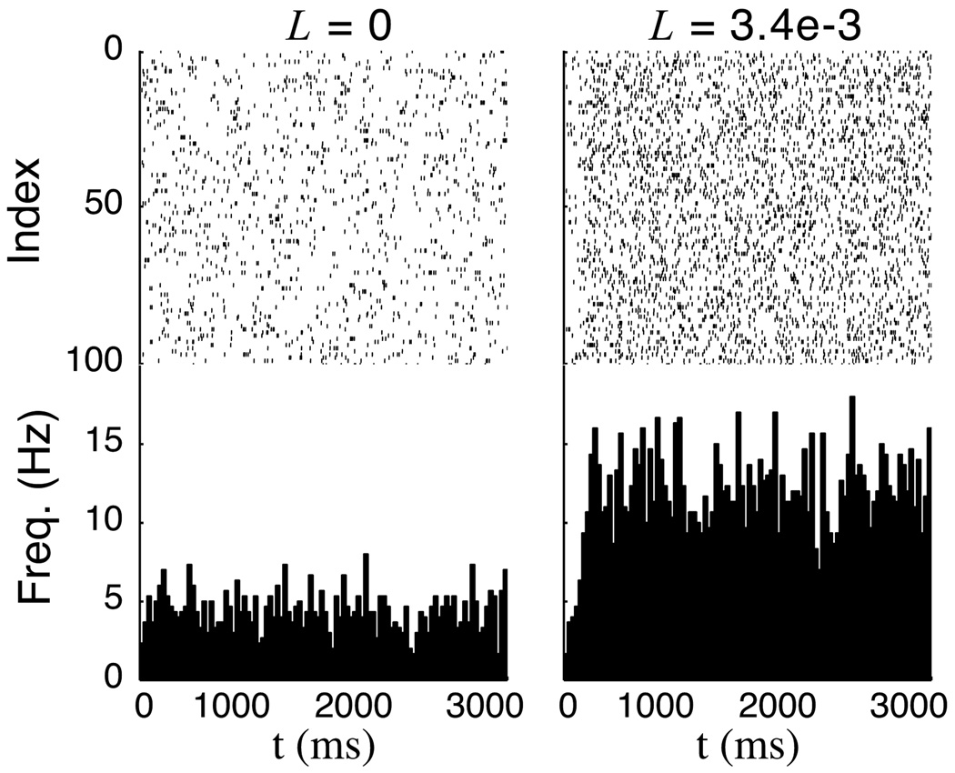
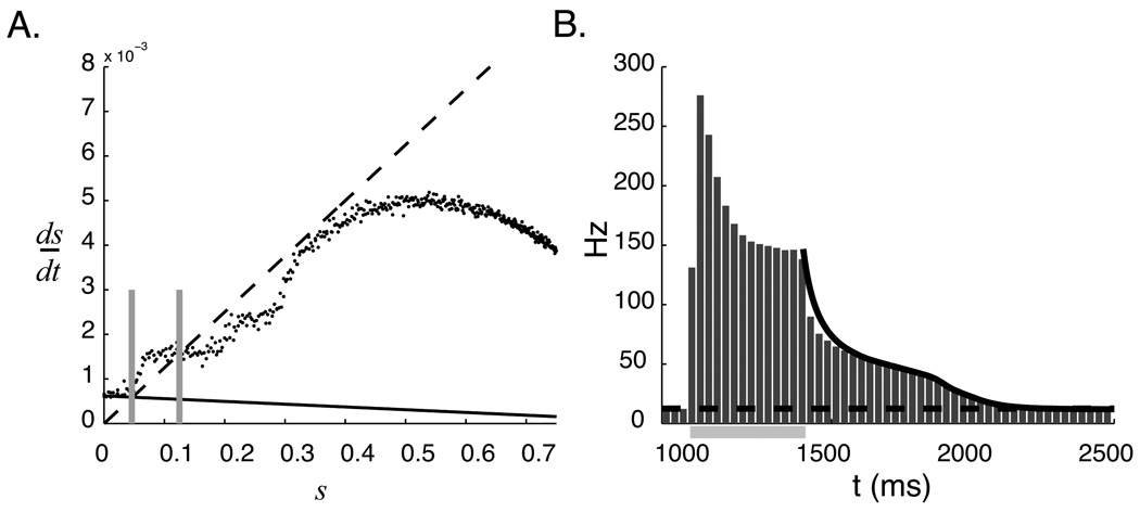
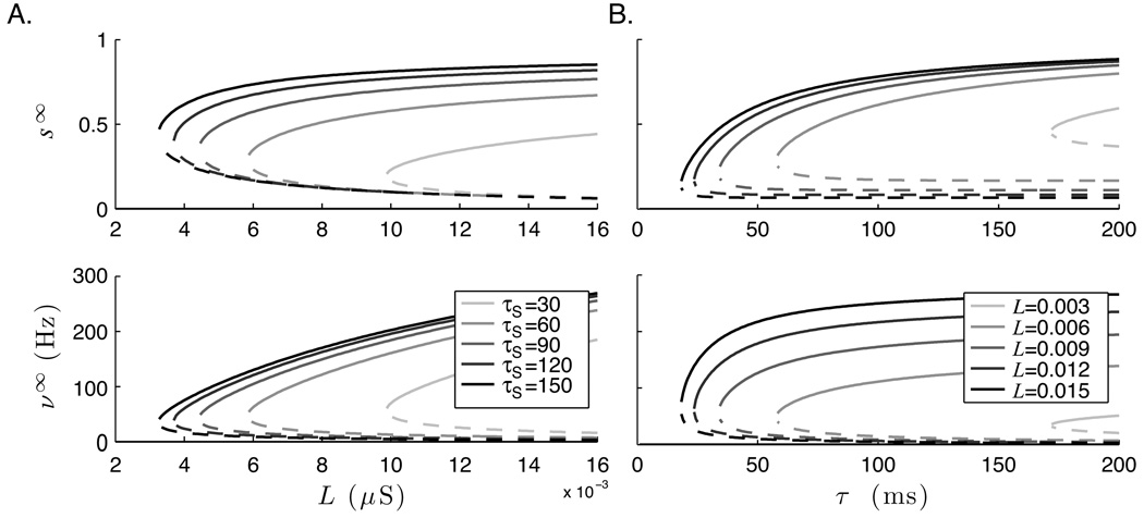
Despite the vital importance of our ability to accurately process and encode temporal information, the underlying neural mechanisms are largely unknown. We have previously described a theoretical framework that explains how temporal representations, similar to those reported in the visual cortex, can form in locally recurrent cortical networks as a function of reward modulated synaptic plasticity. This framework allows networks of both linear and spiking neurons to learn the temporal interval between a stimulus and paired reward signal presented during training. Here we use a mean field approach to analyze the dynamics of non-linear stochastic spiking neurons in a network trained to encode specific time intervals. This analysis explains how recurrent excitatory feedback allows a network structure to encode temporal representations.

Figure 1

Temporal representations created by RDE. A. Neurons in the recurrent layer of our network model are stimulated by retinal activation via the LGN. L is the matrix defining lateral excitation. B. With a linear neuron model, time is encoded by the exponential decay rate of an activity variable V. C. In the spiking neuron model, evoked activity (shown by spike rasters, where each row represents a single neuron in the network, and the resultant histogram) in a responsive sub-population of the network persists until the time of reward. In both models, the stimulus is active during the period marked by the gray bar and the reward time is indicated by the dashed line. See (Gavornik et al., 2009) for details of learning with RDE.

Figure 2

Input-Output relationship of an IF neuron. A. The analytical ϕ curve (black line) calculated using MFT analysis (equation 12) with W = 3.4e-3 μS compared to numerically generated estimates of the output rate ν (symbols). K indicates the number of independent synapses driving activity in the numerically simulated neuron; individual synaptic weights are scaled by K so that the cumulative synaptic weight is constant for each of the three cases shown (K=1,10,100). As K increases, the numerical approximations approach the analytical curve. Note that in the model described in section 3, K=N=100 for the recurrent synapses. Deviations exist primarily in the low frequency input region where output is driven by fluctuations (see equations 13 and 14). B. The analytical solution (solid lines) compares well with numerical results (plus signs, K=100) for values of W ranging from 1.5e-3 μS (light gray) to 6.0e-3 (black). All parameters are as listed in section 3.

Figure 3

Relaxation dynamics of reduced mean field model. A. Source (solid curves) and sink (black dashed line) components of the pseudo-steady state equation (eq. 15) for three values of the excitatory recurrent weight. L = 2.2e-3 μS (light gray), 4.4e-3 μS (gray), and 8.8e-3 μS (black). B. Resulting dynamics. Critical slowing occurs when recurrent weights move the positive component sufficiently close to the negative component. A stable “up” state appears if the weights grow large enough that the lines intersect.

Figure 4

Pseudo steady-state model prediction compared to full I&F model. The plots above show trajectories generated by solving the pseudo steady-state equation compared to values extracted from the full spiking network model for two values of lateral recurrent weights. In the top plot, the solid lines are the trajectories predicted by integrating equation 15 and the stars indicate the average synaptic activation variable of 100 neurons participating in a temporal representation over a single run. In the bottom plot, the bars show the PSTH of the spiking neurons overlaid with the spike frequencies predicted from the mean-field theory (dashed black lines). The initial condition s(0)=0.625 was taken from the simulations of the complete network at the end of the stimulus period.

Figure 5

A. The duration of encoded time estimated by integrating s from 1 to 0.05. With the parameters used in this paper, encoding times above approximately 1.5 s becomes difficult due to the sensitivity of the encoded representation to very small changes in L. B. Invariance of temporal representation to stimulus magnitude. This plot shows the pseudo-steady state system response of a single “trained” network with initial conditions representing different stimulus levels. If vigorous stimulation drives the network to a sufficiently high level, the temporal report is approximately the same (light gray lines). An intermediate stimulus show a degraded temporal report (gray), and the response to low-level stimulation (black) is identical to the report of an isolated neuron. Temporal reports above a threshold value of s (0) ≈ 0.45 are very similar.

Figure 6

Spontaneous activity in the full network model. Here, spontaneous spiking in the recurrent layer is driven by stochastic feed-forward synapses each with maximal conductance of 2.1e-2 μS and a synaptic time constant of 10 ms. The synapses are driven by independent poisson spikes arriving at and average rate of 12.5 Hz. These plots (raster plots for each neuron in the recurrent layer over a binned histogram showing firing rate) show that the spontaneous activity rate driven by these inputs increases from approximately 4 Hz in a network with no recurrent connections to ≈ 12 Hz when the total value of L=3.4e-3 μS. A similar increase in the spontaneous firing rate was also seen in the experimental data.

Figure 7

Accounting for changes in spontaneous activity. A. The sink (dashed black line) and source curves for the cases that L = 0 (solid black line) and L = 3.4e-3 μS (black points, numerical estimates made over multiple simulation runs). Spontaneous activity occurs at, and is set by, the intersection of the source and sink curves (marked for both L values by two vertical gray lines). This plot shows that the spontaneous activity level increase from 4.2 Hz (s = 0.046) to 12.5 Hz (s = 0.125) as a function of recurrent excitation. B. Dynamics during the decay period (solid black line) calculated using this numerical curve and equation 15 match those seen in the full network model (gray bars show spike frequency in the network averaged over 50 runs over the period of stimulation, marked by the light gray bar, and temporal report). The dashed line marks the spontaneous activity level estimated from the full network and matches the value predicted from A.

Figure 8

Bifurcation diagrams of the fixed-point values from the pseudo steady-state model (equation 15) demonstrate bistability. Solid lines indicate stable fixed points, and dotted lines indicates unstable fixed points. The top plots shows the synaptic activation variable at steady states (s^∞) and the bottom plots show the resultant firing rate (ν^∞). A. Bistability as a function of lateral recurrent weights (L) over a range of τ_s values. B. Bistability as a function of τ_s for several fixed values of L. With zero spontaneous activity, all solutions have fixed point at s = 0.

References

1. Amit DJ. Modeling brain function : the world of attractor neural networks. Cambridge [England]: Cambridge University Press; 1989. New York, 89015741 Daniel J. Amit. ill. ; 24 cm. Includes bibliographies and index.
1. Amit DJ, Brunel N. Model of global spontaneous activity and local structured activity during delay periods in the cerebral cortex. Cereb Cortex. 1997;7(3):237–252. - PubMed
1. Amit DJ, Gutfreund H, Sompolinsky H. Spin-glass models of neural networks. Phys Rev A. 1985;32(2):1007–1018. - PubMed
1. Barbieri F, Brunel N. Can attractor network models account for the statistics of firing during persistent activity in prefrontal cortex? Front Neurosci. 2008;2(1):114–122. - PMC - PubMed
1. Brody CD, Romo R, Kepecs A. Basic mechanisms for graded persistent activity: discrete attractors, continuous attractors, and dynamic representations. Curr Opin Neurobiol. 2003;13(2):204–211. - PubMed
LinkOut - more resources