An approximately Bayesian delta-rule model explains the dynamics of belief updating in a changing environment

Abstract

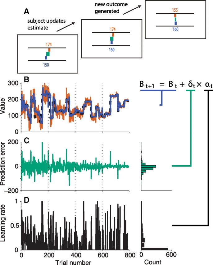
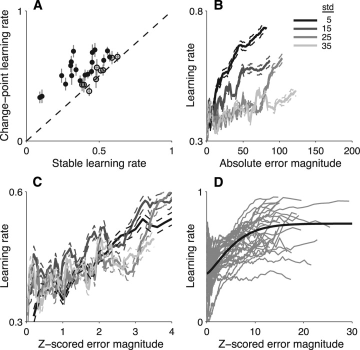
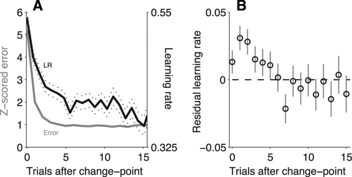
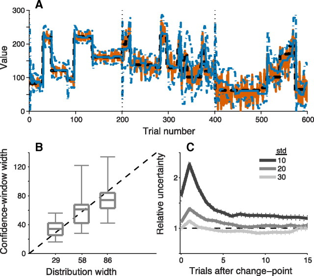
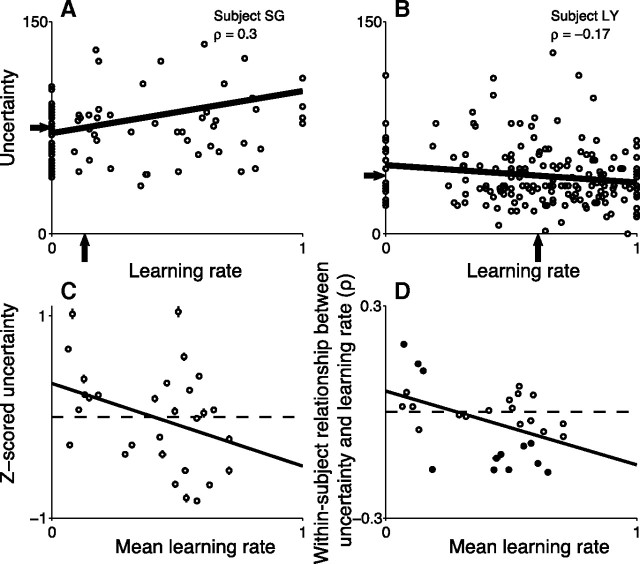
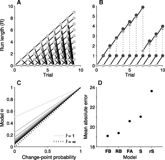
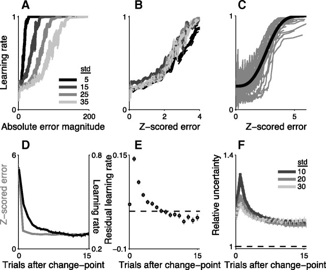
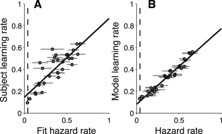
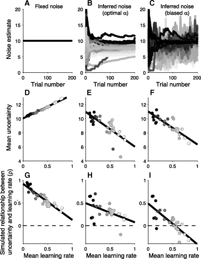
Maintaining appropriate beliefs about variables needed for effective decision making can be difficult in a dynamic environment. One key issue is the amount of influence that unexpected outcomes should have on existing beliefs. In general, outcomes that are unexpected because of a fundamental change in the environment should carry more influence than outcomes that are unexpected because of persistent environmental stochasticity. Here we use a novel task to characterize how well human subjects follow these principles under a range of conditions. We show that the influence of an outcome depends on both the error made in predicting that outcome and the number of similar outcomes experienced previously. We also show that the exact nature of these tendencies varies considerably across subjects. Finally, we show that these patterns of behavior are consistent with a computationally simple reduction of an ideal-observer model. The model adjusts the influence of newly experienced outcomes according to ongoing estimates of uncertainty and the probability of a fundamental change in the process by which outcomes are generated. A prior that quantifies the expected frequency of such environmental changes accounts for individual variability, including a positive relationship between subjective certainty and the degree to which new information influences existing beliefs. The results suggest that the brain adaptively regulates the influence of decision outcomes on existing beliefs using straightforward updating rules that take into account both recent outcomes and prior expectations about higher-order environmental structure.

Figure 1.

Estimation task and its relationship to prediction errors and learning rate. A, Schematized trial of the estimation task. The subject makes a prediction (blue) and is then shown the outcome (red) and the error made in predicting the outcome (teal). After the subject updates his prediction as a fraction of the error, a new outcome is generated. B, An example session. Numbers (red line) are generated from a normal distribution with a variance that is constant within blocks of 200 trials (vertical, dotted lines) and a mean (dashed black line) that changes at random times. The subject's trial-by-trial predictions are shown in blue. C, Trial-by-trial prediction errors from the session in B (actual in red minus prediction in blue). Histogram (right) shows the distribution of prediction errors made over the course of the entire session. D, Trial-by-trial learning rates from the session in B, computed as the fraction of the prediction error used to update the next prediction using a delta rule, as shown. Histogram (right) shows the distribution of learning rates across the entire session.

Figure 2.

Learning rates increased after unexpected errors. A, Mean ± SEM learning rates on trials in which the mean of the generative distribution changed (ordinate) versus on other trials (abscissa; error bars are obscured by the points). Points are data from individual subjects. Filled symbols indicate Wilcoxon test for H₀: equal median learning rates on change-point and non-change-point trials, p < 0.05. B, Learning rate plotted as a function of median absolute error magnitude, averaged using running bins of 150 trials, for four different SDs of the generative distribution, as indicated. Data are averaged across all subjects. Solid and dashed lines indicate mean and SEM, respectively. C, Learning rate plotted as a function of median relative error magnitude, plotted as in B. The relative error magnitude was computed by dividing the absolute error magnitude by the SD of the generative distribution. D, Individual subject learning rates plotted as a function of relative absolute error magnitude (gray lines). The black line indicates a cumulative Weibull function fit to data from all subjects.

Figure 3.

Learning rates decayed slowly after change points. A, Prediction errors (gray, left ordinate) and learning rates (black, right ordinate) plotted as a function of trials after a change point. Solid lines indicate the mean across all subjects and all conditions; dotted lines indicate SEM. B, Learning rate residuals plotted as a function of trials after a change point. Residuals were computed by subtracting the learning rates predicted by the cumulative Weibull fit shown in Figure 2D from the actual learning rates, and thus reflect the portion of learning rate that was not explained by relative error magnitude. Points and error bars are mean ± SEM across all subjects.

Figure 4.

Subjective confidence measurements. A, An example session of the confidence task. Subjects specified a symmetric window (dashed blue lines) around their estimate (solid blue line) that they were 85% certain would contain the next number (red) generated using the current mean (dashed black line) and SD (stable in blocks, indicated by the vertical, dotted lines). B, Box-and-whisker plot (central line is the median, box is the interquartile range, and whiskers are the data range) of the distribution of the mean width of the 85% confidence window computed per subject for each standard-deviation condition. C, Relative uncertainty as a function of trials after a change point. Relative uncertainty was computed by dividing the specified confidence window size by the size of the smallest window capable of including 85% of the probability density in the actual generative distribution (B, x-axis markers). Solid and dotted lines indicate mean and SEM, respectively.

Figure 5.

Relationship between confidence and learning rate. A, B, Trial-by-trial learning rates plotted as a function of uncertainty (confidence-window width) for an example task block (SD, 20) for two different subjects. Solid lines are linear fits. Arrows indicate the mean values of the confidence-window width and learning rate. C, Mean relative uncertainty (computed as the z-scored confidence-window width across all conditions per subject) plotted as a function of mean learning rate. Symbols and error bars are mean ± SEM per subject. The solid line is a linear fit (r = −0.38; p = 0.04). The negative correlation implies that subjects who used higher learning rates tended to be more certain about their predictions. D, Trial-by-trial relationship between relative uncertainty and learning rate per subject (ordinate, computed as Spearman's ρ as in A and B; filled symbols indicate H₀: ρ = 0, p < 0.05; a positive or negative value indicates that the subject tended to use higher or lower learning rates on trials in which they were more uncertain about their previous prediction, respectively) plotted as a function of the average learning rate used by that subject. Symbols and error bars are the mean ± SEM per subject. The solid line is a linear fit (r = −0.44; p = 0.02). The negative correlation implies that subjects who used lower learning rates tended, on average, to have more positive trial-by-trial relationships between uncertainty and learning rate.

Figure 6.

Bayesian model. A, Message-passing algorithm for the full model. Run length (r) refers to the number of data points obtained previously from the current generative distribution. On each trial, the distribution either changes and r is set to zero, or the generative distribution does not change and r is increased by one. After t trials, the algorithm must maintain and update t + 1 predictive distributions (one for each possible r) and the probability distribution across these possible values of r. B, Message-passing algorithm for the reduced model. Instead of considering all possible values of r, the model considers only the possibility that a change point did occur (represented by solid lines from r = 0 to r = 1) or did not occur (represented by all other solid lines). Posterior probabilities of these alternatives are computed according to Bayes' rule, then combined by taking the expected value of the run-length distribution r̂ (small, gray, filled circles). Only a single, approximate predictive distribution is maintained and updated on a trial-by-trial basis. This approach massively reduces complexity and leads the algorithm to take the form of a delta rule (see Materials and Methods). C, Learning rates used by the reduced Bayesian model can be described analytically in terms of r̂ and change-point probability. Lines indicate relationships between learning rate and change-point probability for a given r̂ (increasing for darker lines). The dotted black line reflects the theoretical limit of the function as r̂ goes to infinity. D, Performance of subjects and models. Mean absolute errors made by the full Bayesian model (FB), the reduced Bayesian model (RB), a delta-rule model using the best fixed learning rate possible for each session (FA), subjects (S), and a delta-rule model using subject learning rates in random order (rS) are shown.

Figure 7.

The reduced Bayesian model qualitatively reproduces belief-updating behavior. All plots in this figure depict simulated data using the reduced Bayesian model. One model parameter, the hazard rate, was fit for each block to minimize the difference between model and subject predictions. A, Learning rate as a function of absolute error magnitude for different SDs of the generative distributions, as shown (compare Fig. 2B). B, Learning rate as a function of z-scored error, plotted as in A (compare Fig. 2C). C, Across-subject variability in the relationship between learning rate and z-scored error, simulated by fitting data from different subjects with different hazard rates (gray lines). The black line is the cumulative Weibull fit (compare Fig. 2D). D, Z-scored error (gray, left ordinate) and learning rate (black, right ordinate) plotted as a function of trials after a change point. The solid and dashed lines indicate mean ± SEM (compare Fig. 3A). E, Learning rate residuals plotted as a function of trials after a change point. Residuals were computed by subtracting the learning rates predicted by the cumulative Weibull fit shown in C from the actual learning rates, and thus reflect the portion of learning rate that was not explained by relative error magnitude. Points and error bars are mean ± SEM across all simulated data (compare Fig. 3B). F, Relative model uncertainty (computed as the minimal window containing at least 85% of the probability density in the predictive distribution specified by the model divided by the 85% width of the true generative distribution) plotted as a function of trials after a change point. The grayscale reflects the SD of the given task block, as indicated (compare Fig. 4C).

Figure 8.

Relationship between learning rate and hazard rate. A, Variability in subject learning rates can be described by the hazard rate in the model. Subjects that are fit best by high hazard rate versions of the reduced Bayesian model use higher learning rates, on average. The dashed line indicates the actual average hazard rate for the task. Points and error bars represent the mean and SEM, respectively. The solid line is a linear fit (r = 0.84; p < 0.001). B, Higher hazard rate models tend to use higher learning rates. Points and error bars represent the mean and SEM for all fits to a given subject (across all task blocks). The solid line is a linear fit (r = 0.98; p < 0.001).

Figure 9.

On-line noise inference. Individual variability was simulated by using models that employed the hazard rates fit to individual subject data (see Computing best-fitting hazard rates in Materials and Methods) (in all panels, grayscale represents the different hazard rates, with lighter shades for higher rates). Three models that differed only in their method for computing noise were used to simulate performance. The first, simplest model (left) used the actual SD of the generative distribution. The second model (middle) inferred noise using an on-line algorithm with learning rates that assumed noise was constant over each block of 200 trials (Eqs. 22, 23). The third model (right) inferred noise using the same algorithm as the second model, but with a minimum learning rate that depended on hazard rate (Eq. 24). A–C, Noise estimates from each model over the course of each 200-trial block in which the SD of the generative distribution was equal to 10. D–F, The mean uncertainty estimate for each simulated block of trials plotted as a function of the mean learning rates used in that simulation. Lines are linear fits. Negative relationships in E and F reflect the fact that individuals modeled with higher hazard rates tended to use higher learning rates and infer less noise. G–I, Correlations between uncertainty and learning rate within single simulated task blocks plotted as a function of the mean learning rate simulated for that subject. Lines are linear fits. All models show a negative relationship, but only the third model matches the behavioral data, with low mean learning rates typically corresponding to positive relationships between learning rate and uncertainty, and high mean learning rates typically corresponding to negative relationships between learning rate and uncertainty.

Figure 10.

Hazard rate trade-off. A, Average absolute errors made by subjects one to five trials after a change point plotted as a function of the fit hazard rate from the reduced Bayesian model for each subject (points). The line is a linear regression (r = −0.43; p = 0.02). The negative relationship implies that subjects who used higher hazard rates made better predictions after change points. B, Average absolute errors made by subjects six or more trials after a change point plotted as a function of the fit hazard rate for each subject (points). The line is a linear regression (r = 0.51; p < 0.01). The positive relationship implies that subjects who used lower hazard rates made better predictions during periods of stability.

Figure 11.

Better descriptive models to capture suboptimal performance. A, Although subjects (filled symbols; data are plotted as in Fig. 2A) and the reduced Bayesian model (open symbols) both used higher learning rates after change points than during a stable period, the model tends to show a larger effect. B, Relationship between learning rate and relative error magnitude for subjects (dotted line; the fit from Fig. 2D) and several models fit to subject behavior, as indicated. C, Histogram of the average likelihood weight fit to each subject (Eq. 25, λ). When λ = 0, the model updates beliefs according to a fixed learning rate delta rule. When λ = 1, the model is the reduced Bayesian model. All subjects fell between these two extremes. D, Bayesian information criterion (BIC) for all models in B fit to subject data. Lower values imply better fits, including penalties for additional parameters. Points and error bars are mean ± SEM across subjects. The grayscale and model numbers are as in B.

References

1. Adams RP, MacKay DJ. Cambridge, UK: University of Cambridge Technical Report; 2007. Bayesian online changepoint detection.
1. Behrens TE, Woolrich MW, Walton ME, Rushworth MF. Learning the value of information in an uncertain world. Nat Neurosci. 2007;10:1214–1221. - PubMed
1. Bruder GE, Keilp JG, Xu H, Shikhman M, Schori E, Gorman JM, Gilliam TC. Catechol-O-methyltransferase (COMT) genotypes and working memory: associations with differing cognitive operations. Biol Psychiatry. 2005;58:901–907. - PubMed
1. Corrado GS, Sugrue LP, Seung HS, Newsome WT. Linear-nonlinear-Poisson models of primate choice dynamics. J Exp Anal Behav. 2005;84:581–617. - PMC - PubMed
1. Daw N, O'Doherty J, Dayan P, Seymour B, Dolan R. Cortical substrates for exploratory decisions in humans. Nature. 2006;441:876–879. - PMC - PubMed
Publication types
LinkOut - more resources