Selectivity and tolerance ("invariance") both increase as visual information propagates from cortical area V4 to IT

Abstract

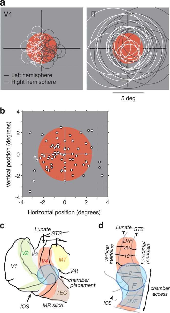
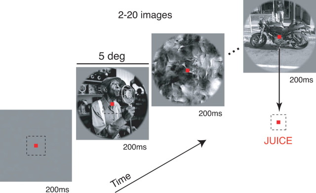
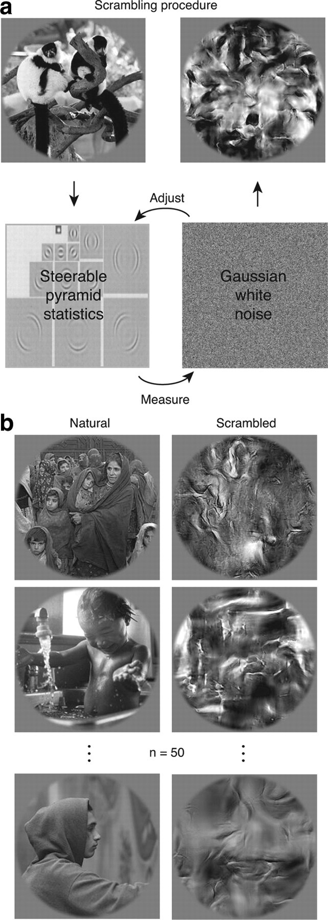
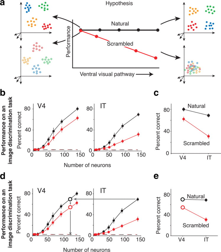
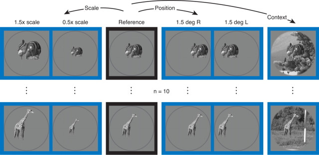
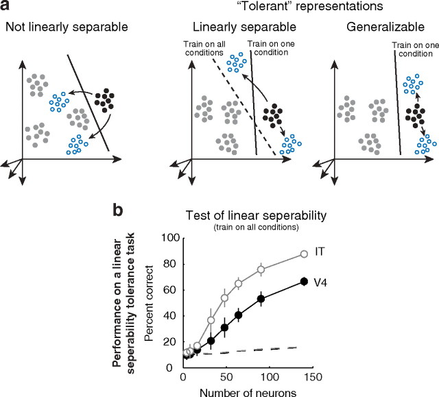
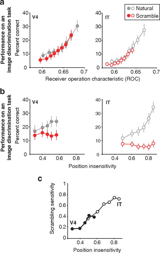
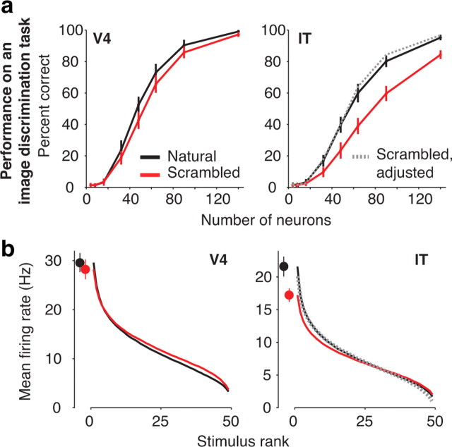
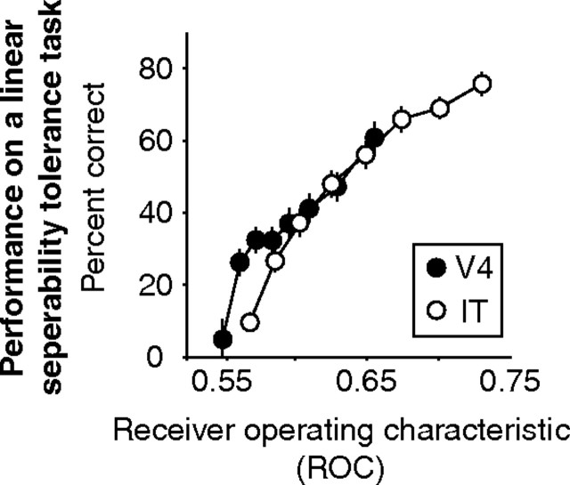
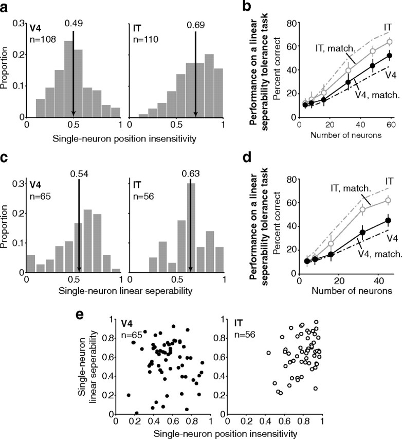
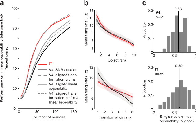
Our ability to recognize objects despite large changes in position, size, and context is achieved through computations that are thought to increase both the shape selectivity and the tolerance ("invariance") of the visual representation at successive stages of the ventral pathway [visual cortical areas V1, V2, and V4 and inferior temporal cortex (IT)]. However, these ideas have proven difficult to test. Here, we consider how well population activity patterns at two stages of the ventral stream (V4 and IT) discriminate between, and generalize across, different images. We found that both V4 and IT encode natural images with similar fidelity, whereas the IT population is much more sensitive to controlled, statistical scrambling of those images. Scrambling sensitivity was proportional to receptive field (RF) size in both V4 and IT, suggesting that, on average, the number of visual feature conjunctions implemented by a V4 or IT neuron is directly related to its RF size. We also found that the IT population could better discriminate between objects across changes in position, scale, and context, thus directly demonstrating a V4-to-IT gain in tolerance. This tolerance gain could be accounted for by both a decrease in single-unit sensitivity to identity-preserving transformations (e.g., an increase in RF size) and an increase in the maintenance of rank-order object selectivity within the RF. These results demonstrate that, as visual information travels from V4 to IT, the population representation is reformatted to become more selective for feature conjunctions and more tolerant to identity preserving transformations, and they reveal the single-unit response properties that underlie that reformatting.

Figure 1.

Experimental design. a, All images were displayed in a 5° diameter aperture located at the center of gaze (red). Expected receptive field locations and sizes for neurons in V4 (Desimone and Schein, 1987; Gattass et al., 1988) and IT (Op De Beeck and Vogels, 2000). To compare these two areas, we targeted V4 neurons such that the population of V4 receptive fields tiled the image. This required recording from both the right (white) and left (dark gray) hemispheres. b, The receptive field locations of a subset (78 of 140) of V4 neurons recorded; dots illustrate their centers relative to the 5° diameter stimulus aperture (gray, monkey 1; white, monkey 2). c, Occipital cortex, illustrating the location of V4 relative to other visual areas, adapted from Gattass et al. (1988). V4 exists on the cortical surface between the lunate sulcus and the STS and extends into the IOS. Approximate chamber placement indicated in cyan. d, Expanded view of V4, also adapted from Gattass et al. (1988). The lower visual field representation (LVF) in V4 exists on the cortical surface, in which receptive field locations move toward the fovea as one traverses ventrally; approximate eccentricities are labeled according to Gattass et al. (1988). At all eccentricities, receptive fields cluster toward the vertical meridian near the lunate and move toward the horizontal meridian as one approaches the STS. The foveal representation, (labeled F) begins at the tip of the IOS. The upper visual field representation (UVF) can be found within the IOS. Given the foveal confluence of V1, V2, and V4 within the IOS, it is not certain that all of the neurons in the upper field were in fact from V4, although the receptive field sizes were more consistent with V4 than either V2 or V1. Cyan illustrates the approximate region that can be accessed via the chamber, which includes both the lower and upper visual field representations. MT, Middle temporal area; TEO, temporal–occipital area.

Figure 2.

The object detection task performed by monkey 2. Each trial began with the monkey looking at a fixation point. After a brief delay, images were presented, in random order, each for 200 ms. At a randomly preselected point in the trial, an image containing a motorcycle appeared. The monkey then had 500 ms to saccade to the response dot to receive a juice reward. In the intervening time, images continued to stream. To ensure that the monkey was performing an object recognition task as opposed to relying on low-level visual cues, the motorcycle was presented at different scales, positions, and on different backgrounds. In addition, novel motorcycle images were introduced each day (supplemental Fig. 3, available at www.jneurosci.org as supplemental material).

Figure 3.

Assessing the ability of a population of neurons to encode an image set by measuring discriminability with a linear population readout. Left, A hypothetical population response for a single presentation of an image (labeled A). After adjusting for latency (see Materials and Methods), spikes were counted in a 200 ms window. The spike counts for the N neurons recorded within a given visual area were combined to form a “response vector” of length N. Right, The response vector exists in an N-dimensional space but is illustrated in the two-dimensional space defined by the responses of neurons 1 and 2 (circled blue dot). Because neurons are noisy, different presentations of the same image produce slightly different response vectors and together all presentations form a “response cloud.” The images producing each response vector are labeled by color. The ability of the population to discriminate between different images is proportional to how far apart the response clouds are in this space. We quantified discriminability using linear classifier readout techniques (see Materials and Methods). This amounted to finding, for each image, the optimal linear hyperplane (shown here as a line) that separated all the responses to that image from all the responses to all other images. After using a subset of the trials to find each hyperplane, we tested discriminability with other trials by looking to see where the response vectors fell. The hyperplane that produced the maximal response (the hyperplane for which the response vector was on the correct side and the farthest from the boundary) was scored as the answer, and performance was measured as the percentage correct on this image identification task. Example correct and wrong answers for presentations of stimulus A are shown (right).

Figure 4.

Scrambling procedure. a, Images were scrambled using a model introduced by Portilla and Simoncelli (2000). Briefly, the procedure begins by computing a number of image statistics. A Gaussian white-noise image is then iteratively adjusted until it has the same number and type of local, oriented elements but presented at random positions within the image (see Materials and Methods). b, Example natural images and their scrambled counterparts. Each set contained 50 images.

Figure 5.

Testing conjunction sensitivity. a, Logic behind the experiment designed to measure conjunction sensitivity. Top left, Response clouds (see Fig. 3) corresponding to the population response to four natural images for an idealized population that encodes local structure within the images. Bottom left, Response clouds for the same population in response to four scrambled versions of the same natural images. In this scenario, scrambling the images activates the population differently, resulting in a repositioning of the response clouds, but the clouds remain a similar distance apart. Top right, Response clouds for an idealized population that encodes specific conjunctions of local structure. Bottom right, Response clouds for the same population in response to scrambled images. In this scenario, destroying the natural feature conjunctions results in the response clouds collapsing toward the origin. b, Performance as a function of the number of neurons for the V4 and IT populations on the discrimination task for the natural (black) and scrambled (red) image sets. Both sets contained 50 images. SE bars indicate the variability (determined by bootstrap) that can be attributed to the specific subset of trials determined for training and testing and the specific subset of neurons chosen. Also shown is chance performance, calculated by scrambling the image labels (dashed lines, ∼2%; see Materials and Methods). c, Performance of the V4 and IT populations for n = 140 neurons. d, In contrast to equating the number of neurons in each population, V4 and IT can be equated via performance on the natural image set; this amounts to limiting the V4 population to 121 neurons compared with 140 neurons in IT. e, Performance of the V4 and IT populations for n = 121 and n = 140 V4 and IT neurons, respectively.

Figure 6.

Images used to compare tolerance in V4 and IT. Ten objects were presented under six different transformed conditions. The reference objects (black) were always presented near the center of the 5° aperture. The transformed conditions (blue) included rescaling to 1.5× and 0.5× at the center position, presentation at 1× scale but shifted 1.5° to the right (R) and left (L), and presentation at the reference position and scale but in the context of a natural background.

Figure 7.

Comparing tolerance in V4 and IT. a, Logic behind the experiment. The analysis begins by training the linear readout to identify the reference objects and then determining how well this representation generalizes across different positions, scales, and context. Middle, We are testing the hypothesis that the ability to generalize across identity-preserving transformations increases along the pathway. Left, More specifically, we expect that neural populations at earlier stages of visual processing will not be capable of generalization because the response clouds for the images presented at different positions, scales, and context will intermingle with the response clouds for other objects, resulting in reduced discriminability. Right, Conversely, we expect that neural populations at later stages of processing will be capable of generalization because the response clouds for the images presented at different positions, scales, and context will remain on the “correct” side of the linear decision boundary. b, To first assess how well the individual images were encoded, performance on the object discrimination task was determined by training and cross-validated testing on different trials of the same images (similar to the black lines in Fig. 5b). Plotted is the mean performance on the object discrimination task (chance, 10%). Error bars indicate SEs (determined by bootstrap) that can be attributed to the specific subset of trials determined for training and testing and the specific subset of neurons chosen. Ref, Reference; B, 1.5× scale (Big); S, 0.5× scale (Small); L, 1.5° shift left; R, 1.5° shift right; BG, presentation on a natural background. Performance was high across all transformations in both V4 and IT. c, Generalization across position for the V4 (left) and IT (middle) populations. Black lines indicate mean performance as a function of the number of neurons when training and testing on the reference objects. Blue lines indicate average performance when asked to generalize across small changes in position (from the reference to 1.5° to the left or right). Dashed lines indicate chance performance (∼10%), calculated by scrambling the image labels (see Materials and Methods). Error bars indicate SEs (determined by bootstrap) that can be attributed to the specific subset of trials determined for training and testing and the specific subset of neurons chosen. Right, Performance of the V4 and IT populations when nearly all recorded neurons (n = 140) from each area are included. d, Generalization capacity for different transformations, calculated as the fractional performance on the generalization task relative to the reference. For example, generalization capacity across small changes in position (the 2 leftmost bars) is calculated as the ratio of the blue and black points in c (right). Large changes in position correspond to the average generalization across 3° transformations (right to left and left to right): small changes in scale correspond to the average generalization from the reference to the 0.5× and 1.5× images; large changes in scale correspond to the average generalization from 0.5× to 1.5× and vice versa; and changes in context correspond to average generalization from objects on a gray to natural background and vice versa.

Figure 8.

A second tolerance test: linear separability. a, Hypothetical representations that perform poorly and well at tests of tolerance. Left, A population representation that will fail to support tolerant object recognition because of a lack of linear separability. Middle, A population representation that can, in principle, support tolerant object recognition, but one for which the generalization test presented in Figure 7 may fail to find it. The linear boundary located by training on the reference condition alone (solid line) fails to separate the response vectors corresponding to different transformations of one object from the response vectors corresponding to the other objects. In this case, a more appropriate linear boundary (dashed line) can be located by training on all transformations simultaneously. Right, A population representation that performs well at tests of tolerance when training on the reference condition alone. b, Performance on an object identification task for the six transformations of each of 10 objects when the linear boundaries were trained on response data from all six transformations simultaneously and tested with cross-validation data in IT (white) and V4 (black). Dashed lines indicate performance when different objects at different transformations are randomly assigned to one another (e.g., object 1 at the reference position and scale paired with object 3 shifted left 1.5° and object 6 at 0.5× scale, etc.).

Figure 9.

The relationship between single-neuron measures and population discriminability for natural and scrambled images. a, Single-neuron ROC computed for natural (gray) and scrambled (red) images as the average pairwise ROC for 50 natural and 50 scrambled images (Fig. 4). Neurons were ranked separately for their average natural and scrambled image ROC, and population performance for natural or scrambled image discrimination was assessed for subpopulations of 48 neurons with neighboring ROC values. The x-axis shows the geometric mean ROC of each subpopulation in V4 (left) and IT (right). The y-axis shows performance on the discrimination task for the natural (gray) and scrambled (red) image sets (Fig. 5). b, Single-neuron RF size measured as the insensitivity of the responses to the objects across changes in position (see Fig. 12a). Neurons were ranked by position insensitivity, and population performance for natural and scrambled image discrimination was assessed for subpopulations of 48 neurons with neighboring position insensitivity values. The x-axis shows the geometric mean position insensitivity of each subpopulation. The y-axis shows performance on the discrimination task for the natural (gray) and scrambled (red) image sets (Fig. 5). c, Scrambling sensitivity, calculated as the ratio of scrambled and natural image performance (taken from b), subtracted from one and plotted for subpopulations of 48 neurons with neighboring position insensitivity values.

Figure 10.

SNR differences can account for decreased scrambled image discriminability in IT. a, Natural (black) and scrambled (red) image discriminability when the mean firing rate of each neuron to each image is preserved but trial-to-trial variability is replaced with a Poisson process. Also shown is discriminability after adjusting the mean dynamic range of the IT population response to scrambled images to match the mean dynamic range of the population response to natural images (gray dashed; see b). b, Mean dynamic range for natural (black) and scrambled (red) images, computed by averaging over the responses of all neurons after organizing the responses of each neuron in rank order. Points on the left of each plot show mean and SE of firing rate to the most effective natural (black) and scrambled (red) stimulus, averaged across all neurons (to indicate error for firing rates of stimulus rank 1). Gray dashed lines indicate the mean dynamic range after the responses of each IT neuron to scrambled images are adjusted with a multiplicative factor and an offset to match the IT responses to natural images (see Results).

Figure 11.

The relationship between single-neuron ROC and population tolerance. Single-neuron ROC computed as the ROC for discriminations between all six transformations of the best object of a neuron (defined by the highest firing rate after averaging across all transformations) and all six transformations of the nine other objects. Neurons were ranked by their ROC values, and population performance for the linear separability test of tolerance (see Fig. 8b) was assessed for subpopulations of 48 neurons with neighboring ROC values in V4 (black) and IT (white). The x-axis shows the geometric mean ROC of each subpopulation. The y-axis shows population performance for the linear separability test of tolerance (see Fig. 8b).

Figure 12.

Single-neuron correlates of population tolerance. a, Position insensitivity of the V4 and IT population based on the responses to the objects presented at the center of gaze, 1.5° to the left of center, and 1.5° to the right (see Fig. 6). For each neuron, a receptive field profile was computed as the average response at each position to all objects that produced a response significantly differently from baseline at one or more positions (t test, p < 0.05; 108 of 140 neurons in V4 and 110 of 143 neurons in IT). After normalizing the receptive field profile to 1 at the preferred position, we quantified position sensitivity as the average fractional response at the two non-optimal positions. Arrows indicate means. b, Performance on the same object identification task presented in Figure 8b but for an IT and V4 population that are matched for position insensitivity. Each subpopulation was chosen by randomly sampling the maximal number of entries in each histogram bin in a that overlapped. Solid lines indicate populations matched in this way in IT (white) and V4 (black). Dashed lines indicate populations that passed the significance test for at least one object but when not equated for position sensitivity (all the entries in the histograms of a). c, Single-neuron linear separability index measured as the correlation between the actual responses of the neuron and the predicted responses assuming independence between the responses to the 10 objects and each of six transformed conditions (see Fig. 6 and Materials and Methods). For this analysis, only neurons that responded significantly differently from baseline to at least one object under at least two transformed conditions were included (V4, n = 65 of 140; IT, n = 56 of 143). Arrows indicate means (V4, 0.54; IT, 0.63). d, Similar to b, performance on the same object identification task presented in Figure 8b but for an IT and V4 population that are matched for their linear separability index (n = 45; mean V4, 0.586; IT, 0.588). Solid lines indicate populations matched in this way in IT (white) and V4 (black). Dashed lines indicate populations that passed the significance test for at least one object but when not equated for single-neuron linear separability (all the entries in the histograms of c). e, Plots of position insensitivity versus linear separability index in V4 (left) and IT (right).

Figure 13.

Receptive field differences can account for higher population tolerance in IT. a, Performance of the V4 (black) and IT (red) populations on the invariant object recognition task described for Figure 8b after equating V4 and IT for SNR (responses of each V4 cell were rescaled by 0.78, and trial-to-trial variability of both V4 and IT neurons was simulated by a Poisson process). Additional transformations to the V4 population include the following: aligning the V4 transformation profile to match the average IT transformation profile (gray dashed; see Results; b); aligning the average V4 single-neuron linear separability to match the average in IT (gray solid; see Results; c); aligning both the V4 transformation profile to match the average IT transformation profile and aligning the average V4 single-neuron linear separability to match the average in IT (gray dot-dashed). b, Top, Average across the population of the rank-order response to all objects computed after averaging across all six transformations. Bottom, Average across the population of the rank-order response to all six transformations computed after averaging across all 10 objects. V4, Black; IT, red; gray dashed, V4 after aligning the transformation rank profile to match IT. Colored regions indicate mean ± 1 SE. c, Single-neuron linear separability histograms computed after manipulating the internal structure of the V4 neurons' 10 object × 6 transformation response surface to match the average single-neuron linear separability in IT (see Results). Arrows indicate means.

References

1. Anzai A, Peng X, Van Essen DC. Neurons in monkey visual area V2 encode combinations of orientations. Nat Neurosci. 2007;10:1313–1321. - PubMed
1. Baker CI, Behrmann M, Olson CR. Impact of learning on representation of parts and wholes in monkey inferotemporal cortex. Nat Neurosci. 2002;5:1210–1216. - PubMed
1. Brincat SL, Connor CE. Underlying principles of visual shape selectivity in posterior inferotemporal cortex. Nat Neurosci. 2004;7:880–886. - PubMed
1. Britten KH, Shadlen MN, Newsome WT, Movshon JA. The analysis of visual motion: a comparison of neuronal and psychophysical performance. J Neurosci. 1992;12:4745–4765. - PMC - PubMed
1. Denys K, Vanduffel W, Fize D, Nelissen K, Peuskens H, Van Essen D, Orban GA. The processing of visual shape in the cerebral cortex of human and nonhuman primates: a functional magnetic resonance imaging study. J Neurosci. 2004;24:2551–2565. - PMC - PubMed
Publication types