Linear hypergeneralization of learned dynamics across movement speeds reveals anisotropic, gain-encoding primitives for motor adaptation

Abstract

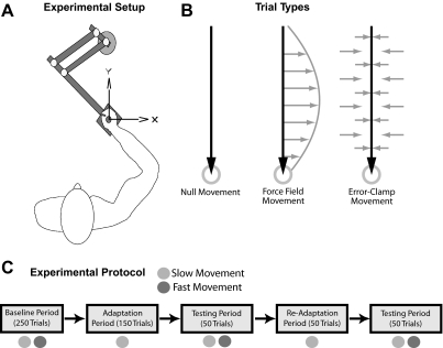
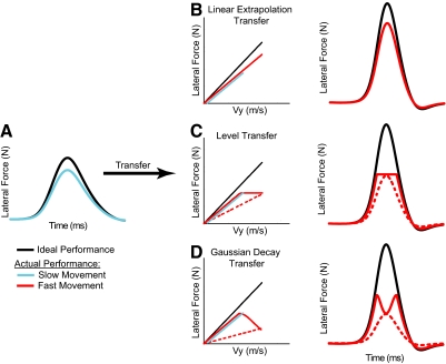
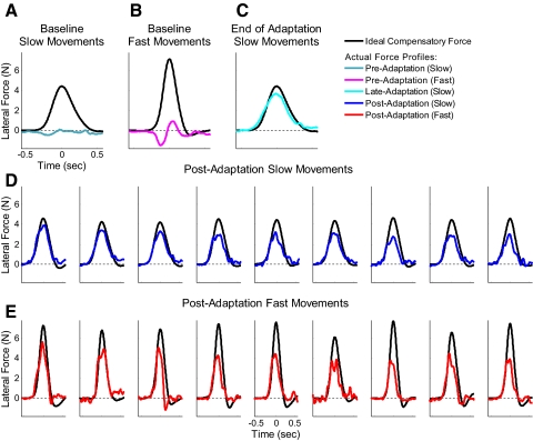
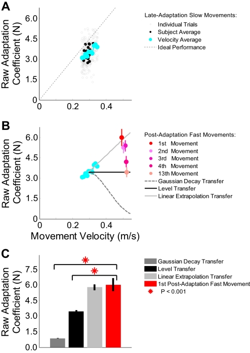
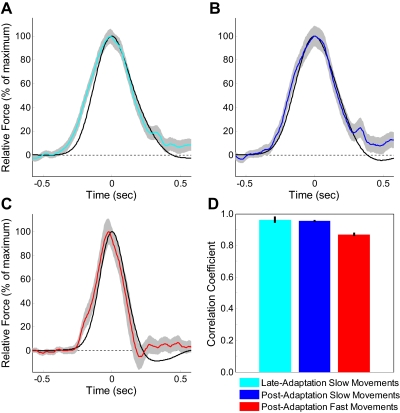
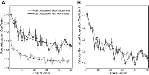
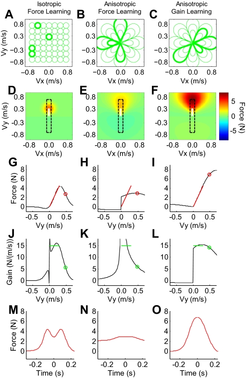
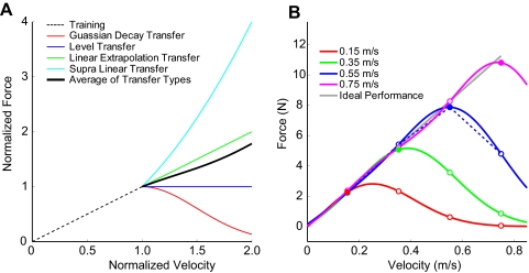
The ability to generalize learned motor actions to new contexts is a key feature of the motor system. For example, the ability to ride a bicycle or swing a racket is often first developed at lower speeds and later applied to faster velocities. A number of previous studies have examined the generalization of motor adaptation across movement directions and found that the learned adaptation decays in a pattern consistent with the existence of motor primitives that display narrow Gaussian tuning. However, few studies have examined the generalization of motor adaptation across movement speeds. Following adaptation to linear velocity-dependent dynamics during point-to-point reaching arm movements at one speed, we tested the ability of subjects to transfer this adaptation to short-duration higher-speed movements aimed at the same target. We found near-perfect linear extrapolation of the trained adaptation with respect to both the magnitude and the time course of the velocity profiles associated with the high-speed movements: a 69% increase in movement speed corresponded to a 74% extrapolation of the trained adaptation. The close match between the increase in movement speed and the corresponding increase in adaptation beyond what was trained indicates linear hypergeneralization. Computational modeling shows that this pattern of linear hypergeneralization across movement speeds is not compatible with previous models of adaptation in which motor primitives display isotropic Gaussian tuning of motor output around their preferred velocities. Instead, we show that this generalization pattern indicates that the primitives involved in the adaptation to viscous dynamics display anisotropic tuning in velocity space and encode the gain between motor output and motion state rather than motor output itself.

Fig. 1.

Experimental setup and protocol. A: subjects sat in front of a computer display and made reaching movements toward and away from the body while holding the handle of a robotic manipulandum that applied forces to the hand. B: there were 3 trial types: null trials, force-field trials, and error-clamp trials. The motors of the manipulandum were turned off for null trials. During force-field trials, the motors were used to produce forces on the hand (gray arrows) that were proportional in magnitude and perpendicular in direction to the velocity of hand motion (black arrow). Forces were determined as a function of hand velocity: f = Bv. During error-clamp trials, the robot motors were used to constrain movements in a straight line toward the target by counteracting any motion perpendicular to the target direction. C: timeline of the experiment. Only slow movements were cued during the adaptation periods, whereas a mixture of both fast and slow movements was cued during the baseline and testing periods.

Fig. 2.

Comparison of predicted generalization patterns for different mechanisms of transfer. The traces in the 1st and last column represent lateral force profiles (lateral force vs. time) associated with force-field adaptation during point-to-point movements: ideal (black) and predicted (colored). The middle column plots the same lateral forces vs. movement velocity. A: typical performance during slow movements after training. Subjects typically produced force patterns that were close to 80% of the ideal patterns, which would fully compensate the force field. We compared several possible mechanisms for transfer of adaptation from slow (blue trace) to fast (red traces) movements. B: linear extrapolation transfer: adaptation remains at 80% of the ideal pattern and the amount of exerted force increases with movement velocity in the same relationship learned during training; C: level transfer: force-level levels off (solid line) or is scaled (dashed line) so that the maximum exerted force at the maximum movement velocity is the same as the force exhibited during adaptation; D: Gaussian decay transfer: force-level decays (solid line) or is scaled (dashed line) in a Gaussian manner for movement velocities beyond those experienced during training. Note that the blue lines in the 2nd column have been shifted slightly to the right to allow the red traces beneath them to be more visible.

Fig. 3.

Evolution of force profiles associated with motor adaptation during the baseline, training, transfer, and decay periods of the experiment. Lateral force patterns for (A) slow movements and (B) fast movements before the adaptation period and (C) late in the adaptation period after adaptation levels had reached asymptote of ∼80% of the ideal force. Lateral force patterns for (D) the 1st 9 slow trials and (E) the 1st 9 fast trials during the postadaptation period are displayed in the bottom 2 rows. The black trace in each panel is the ideal compensatory force pattern based on the force field perturbation that we applied, whereas the actual lateral force patterns we measured in each condition are represented by colored traces. Note the substantial transfer of adaptation to the fast movements in the postadaptation block and the parallel patterns of decay for the slow and fast movements during this block.

Fig. 4.

Raw adaptation coefficients during training and transfer. A: the unfilled gray circles represent the raw adaptation coefficients for the final 5 movements during the adaptation period for all subjects. The filled black circles indicate the average raw adaptation coefficient and movement velocity for each subject. The blue circles are the average raw adaptation coefficients binned by movement velocity. Ten velocity bins are shown, ranging from 0.25 and 0.35 m/s. B: the blue circles display the same data shown in A. The 3 different lines represent different generalization functions: linear extrapolation transfer (light gray), level transfer (black), and Gaussian decay transfer (dark gray, dashed). The red and pink circles show the mean raw adaptation coefficient and velocity for fast movements made during the postadaptation period. The vertical lines represent SE. C: comparison of the raw adaptation coefficient for the 1st fast movement postadaptation with predictions for 3 different mechanisms for generalization. The error bars show SE.

Fig. 5.

Comparison of the shapes of actual and ideal force profiles for slow and fast movements. To examine the shape of each force profile independent of its magnitude, we normalized each by its maximum. Force profiles shapes are shown for (A) slow movements near the end of the adaptation period and (B) slow and (C) fast movements in the postadaptation period. In each panel, the black trace is the ideal compensatory force, the colored traces represent the actual force produced by subjects, and the gray shaded region represents the SE around the latter. D: correlation coefficients for the data presented in A–C. The vertical black bars represent SE.

Fig. 6.

Parallel decay of performance in the postadaptation period for fast and slow movements. A: decay of raw adaptation coefficients as a function of trial number. The black dashed lines are the exponential fits to the data (with time constants of 11.4 and 10.3 trials for fast and slow movements, respectively). B: velocity-normalized adaptation coefficients for the same data presented in A. Data for fast movements are shown in dark gray and slow movements in light gray. The error bars represent SE across subjects.

Fig. 7.

Comparison of adaptation generalization for different motor primitive coding schemes. Shown is the comparison of the 3 different hypothetical configurations of the neural bases (each column) used to simulate the generalization of adaptation to novel movement speeds. The configurations were different in the relationship learned between movement speed and force during adaptation [either an absolute force-velocity (A and B) or force gain-velocity relationship (C)] and arrangement in movement velocity space [either isotropic (A) or anisotropic with differential tuning across magnitude vs. direction (B and C)]. (Note that the basis element illustrations in A–C show contours at the 1-sigma point and only a 4th of the elements are shown to reduce visual overcrowding. The 1-sigma point for the basis elements in both anisotropic primitive simulations was at the origin. Selected bases are highlighted to clarify their shape in velocity space.) In all cases, the relationship learned by the bases during adaptation decayed in a Gaussian manner as the movement velocity moved away from the center of the tuning curve. D–F: the pattern of adaptation (amount of mid-movement force) generalization to different movement velocities for the 3 configurations. The heat map represents the generalization of adaptation in terms of lateral force (N). Note that the color bar alongside F applies to the entire row. The white lines represent the region of velocity space over which the force-field is trained for each model (v_X = 0 ms, v_Y = 0–0.3 m/s). The next 2 rows show the learned force-velocity (G–I) and force gain-velocity relationships (J–L) along the slice of velocity space corresponding to the movement direction experienced during the training (v_X = 0, v_Y = −0.7 to 0.7 m/s, the range enclosed by the black dashed-line rectangle). The red and green lines in these panels highlight the relationships between force and velocity, or force gain and velocity that were trained, corresponding to the white line regions in D–F. Note that the red lines extend from the origin with a slope of 15 Ns/m = B, whereas the green lines have a constant value of 15 Ns/m over the range of 0–0.3 m/s for v_Y. The red and green circles show the extent to which the learning predicted by each model would generalize to the untrained, high-speed movements, we observed during the initial high-speed testing trial (v_Y = 0.49 m/s) to facilitate comparison of these modeling results with the data shown in Fig. 4. The spikes in the black trace in J and K are the result of division by 0 in determining the force gain (F/v_Y) at movement speeds near 0. The bottom row (M–O) shows the resulting lateral force patterns for the 3 different primitive configurations at the initial transfer speed (v_Y = 0.49 m/s).

Fig. 8.

Issues with previous work. A: illustration of the test-period force-fields in Goodbody and Wolpert (1998). During the 384-trial test period of experiment 1 in this study, 75% of trials called for slow movements in a linear viscous force-field with a force-velocity relationship depicted by the black dashed line. The remaining trials consisted of 24 high-speed (double speed) test movements in each of 4 force-fields. These 4 force-fields shared the same linear force-velocity relationship depicted by black dashed line at low speeds but diverged according to the force-velocity relationships shown in the colored traces. The mean of these force-fields is represented by the thick black curve. If experience with the 96 high-speed test trials affected estimated generalization pattern, the effect should reflect the mean force-fields experienced, which is just below linear transfer. B: simulated transfer patterns with the isotropic basis elements used in Francis (2008). The various colored traces show simulated generalization from trained movement speeds 0.15, 0.35, 0.55, and 0.75 m/s. ●, maximum movement speed during training for each trace; ○, generalization to each of these cardinal speeds. Francis (2008) presents simulation of generalization only from 0.55 m/s to the other cardinal speeds—represented here by the blue dashed line. This single simulation matches the experimentally estimated transfer results in Francis (2008) from all 4 movement speeds. However, the simulations of generalization from the other movement speeds, which were not presented in Francis (2008), yield very different transfer patterns, inconsistent with the experimentally estimated transfer results.

References

1. Bastian AJ. Understanding sensorimotor adaptation and learning for rehabilitation. Curr Opin Neurol 21: 628–633, 2008 - PMC - PubMed
1. Bedford FL. Perceptual and cognitive spatial learning. J Exp Psychol Hum Percept Perform 19: 517–530, 1993 - PubMed
1. Bruce CJ, Goldberg ME. Primate frontal eye fields. I. Single neurons discharging before saccades. J Neurophysiol 53: 603–635, 1985 - PubMed
1. Bruce CJ, Goldberg ME, Bushnell MC, Stanton GB. Primate frontal eye fields. II. Physiological and anatomical correlates of electrically evoked eye movements. J Neurophysiol 54: 714–734, 1985 - PubMed
1. Churchland MM, Santhanam G, Shenoy KV. Preparatory activity in premotor and motor cortex reflects the speed of the upcoming reach. J Neurophysiol 96: 3130–3146, 2006 - PubMed
Publication types
LinkOut - more resources